NumPy Exercises#
import numpy as np
np.zeros(3, dtype=int)
np.ones((2, 3))
np.empty((3, 2, 3), dtype=float)
Exercise 1#
Create a 3D array of integers, 2 x 2 x 3, filled with the number 10
A = ...
Exercise 2#
Create a 2D array of integers, 5 x 6, where each item is the product of its row and column:
A = ...
Suggestion: Use for example np.ndindex
Write help(np.ndindex) to see its docstring.
Exercise 3#
Make a square wave \(u^0\):
length = 64
where every 8 elements is either 0 or 1
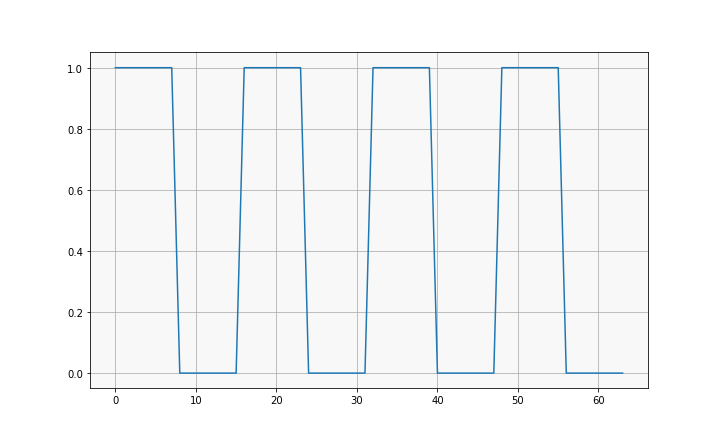
Bonus: 2D!
64 x 64, floats
where every 8 rows and columns is either 1 or 0
%matplotlib inline
import matplotlib.pyplot as plt
u0 = ...
Physics!#
The heat equation is often used for blurring:
We use our square wave as initial solution: $\( u = u^0(x) \quad \text{ at } t=0, \)\( and fix the value of \)u$ at the left and right endpoints:
Take \(I = (0, N)\) and \(T = (0,M)\).
We now \(discretize\) the heat equation as follows $$
$\( where \)u_i^n\( means \)u\( at \)x_i=i\( and \)t=n$
Exercise 4:#
Implement a number of steps of the heat equation.
def heat(u0, time_steps=1):

    u_n = u0 # u_n is the solution at the previous time step
             # we initialize it as u0

    for i in range(time_steps):

        # Apply our discretization!
        u_n1[...] = ....

        # Assign u_n1 as previous solution
        # and proceed to next time step
        u_n = u_n1
    return u_n1

# Plot the solution
x = range(64)
plt.plot(x, u, label="square")
plt.plot(x, heat(u), label="heat(1)")
plt.plot(x, heat(u, 10), label="heat(10)")
plt.plot(x, heat(u, 50), label="heat(50)")
plt.legend(loc=0)
Suggestions:
Use a for loop to iterate through range(N). You can then access elements to the left as u_n[i-1] and to the right as u_n[i+1]
Splice the arrays together. For example, u_n[1:-1] will return all elements of u_n except the left and right endpoints
Exercise 4 bonus:#
In two dimensions, the stencil reads $$
$$
Implement the discretized heat equation in 2D.
Break??#
Exercise 5#
The dot product \(u \cdot v\) for vectors is defined as the cumulative sum of the elementwise product of \(u\) and \(v\):
Part 1: implement the dot product for any two Python iterables
def dot(u, v):
    result = 0

    ...

    return result
N = 100
u = np.arange(N)
v = np.arange(N)

dot(u, v)
Part 2: Measure how long it takes to call your function for iterables of sizes 1000 - 1,000,000
Suggestion: Use tic and toc as below
import time

tic = time.perf_counter()
time.sleep(0.1)
toc = time.perf_counter()
duration = toc - tic
print(f"sleep(0.1) took {duration:.4f}s")
for N in [1000, 10_000, 100_000, 1_000_000]:
    ...

    r = dot(u, v)

    ...

    print(f"N={N:8}, {1000 * (toc-tic):8.2f}ms")
Numpy has its own builtin dot function:
np.dot(u, v)
This is also called via the matrix multiplication operator @:
u @ v
How does numpy’s dot function perform?
for N in [1000, 10_000, 100_000, 1_000_000]:
    ...
    u = np.arange(N)
    v = np.arange(N)
    r = np.dot(u, v)
    ...
    print(f"N={N:8}, {1000 * (toc-tic):8.2f}ms")
Plotting#
%matplotlib inline
import matplotlib.pyplot as plt
For basic plots, plt.plot takes an x list or array and a y list or array
and plots them on a linear scale:
For certain kinds of data, a linear scale isn’t a great fit:
x = [1, 10, 100, 1_000, 10_000, 100_000]
x_squared = np.array(x) ** 2

plt.subplot(1, 2, 1)
plt.plot(x, x_squared, "-o")
plt.title("  x^2 with linear plot")

plt.subplot(1, 2, 2)
plt.loglog(x, x_squared, "-o")
plt.title("  x^2 with loglog plot")
The slope on a linear scale is \(\frac{y}{x}\). The slope on a log-log scale is \(\frac{log(y)}{log(x)}\).
Exercise 6#
collect timings for your dot product and numpy’s dot for a range of lengths up to \(\sim10^6\), and plot:
a separate line for each implementation on one plot, and
a single line showing numpy performance relative to yours
Think about what axis scale is most appropriate for your data
my_times = []
numpy_times = []
relative_performance = []

Ns = [1000, 10_000, 100_000, 1_000_000]

for N in Ns:
    u = np.arange(N)
    v = np.arange(N)

    ...

plt.loglog(Ns, numpy_times, label="np")
plt.loglog(Ns, my_times, label="mine")
plt.legend()
plt.xlabel("N")
plt.ylabel("time")