Numerical computations with NumPy#
Imaging a black hole#

Event Horizon telescope#
The Event Horizon telescope is a collection of eight elescopes that together image the universe with unprecedented resolution. It has an angular resolution of 20 micro-arcseconds - enough to read a newspaper in New York from a sidewalk café in Paris.
Information overload#
Each day this telescope generates over 350 terabytes of observations. Postprocessing this data was a huge challenge.
Numpy was instrumental for this postprocessing.
Code is available in the eht-imaging package. See the eht-imaging homepage for more details or ethim@pypi for installation instructions.
Python is fast to write …#
… but can be slow to run.
In particular, loops over large data structures might be very slow:
for i in range(len(A)):
    A[i] = ...
NumPy enables efficient numerical computing in Python#
The core of NumPy is well-optimized C code.
It provides the flexibility of Python with the speed of compiled code.
Numpy is well worth learning#
NumPy is the de facto standard in Python, and today even is part of interoperability with other languages (R, Julia, etc.).
It is used in libraries such as Pandas, SciPy, Matplotlib, scikit-learn and scikit-image.
Contents#
A first taste of NumPy
Creating arrays
Indexing/slicing arrays
Performance considerations
Plotting
More info#
The NumPy quickstart (https://docs.scipy.org/doc/numpy/user/quickstart.html)
Scientific Computing Tools for Python (https://www.scipy.org)
Scipy Lecture Notes (https://scipy-lectures.org)
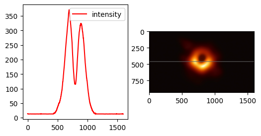
A taste of NumPy#
Plot the intensity of the black hole image across a line.
from PIL import Image

im = Image.open("figs/blackhole.jpg")

# Load pixel data as np array
import numpy as np

data = np.asarray(im, dtype="uint32")

ny, nx = data.shape[:2]  # number of pixels in x and y direction

print(f"Shape = {nx, ny}")

data[0][:3]
Shape = (1600, 932)
array([[11,  5,  5],
       [11,  5,  5],
       [11,  5,  5]], dtype=uint32)
Compute intensity#
The data array gives the RGB tuple of each pixel.

# Get pixel values along x-axis centerline
line_pixels = data[:][ny // 2]

red = line_pixels[:, 0]
blue = line_pixels[:, 1]
green = line_pixels[:, 2]

# compute intensity by squaring RGB values
intensity = (red**2 + blue**2 + green**2) ** 0.5
Then plot!
import matplotlib.pyplot as plt

fig, axs = plt.subplots(1, 2, figsize=(6, 3))

axs[0].plot(intensity, color="red", label="intensity")
axs[0].legend()

# visualize line in image
im_copy = im.copy()

line_thickness, line_color = 4, (100, 100, 100)

for i in range(0, nx):
    for j in range(-line_thickness, line_thickness):
        im_copy.putpixel((i, ny // 2 + j), line_color)

axs[1].imshow(im_copy)
<matplotlib.image.AxesImage at 0x7fd3fe63f910>
Numpy arrays#
The most basic array type that NumPy provides is ndarray. These are N-dimensional homogenous collections of “items” of the same type.
np.array([5., 10., 11.])
np.array(["a", "b", "c"])
Properties:
Arrays have a fixed size.
Arrays have one associated data type.
Contents of arrays are mutable (values in array can be changed)
Creating NumPy arrays#
Numpy provides convenience functions for creating common arrays:
np.zeros(3)
array([0., 0., 0.])
np.ones((3, 1))
array([[1.],
       [1.],
       [1.]])
np.empty((2, 2)) # uninitialised array. Might contain arbitrary data
array([[263.76136364, 169.19026199],
       [290.01136364, 183.19026199]])
Array with a sequence of numbers#
linspace#
linspace(a, b, n) generates n uniformly spaced
coordinates, starting with a and ending with b
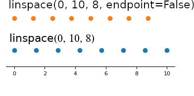
Use endpoint=False to exclude the last point (matches range(start, stop))
np.linspace(-3, 2, num=5)
array([-3. , -1.75, -0.5 , 0.75, 2. ])
np.linspace(-3, 2, num=5, endpoint=False)
array([-3., -2., -1., 0., 1.])
arange#
arange is the numpy equivalent of Python’s range
np.arange(-5, 6, step=2, dtype=float)
array([-5., -3., -1., 1., 3., 5.])
Warning: arange can give unexpected results#
arange’s upper limit may or may not be included!
Demonstration#
Let’s compare
np.arange(8.2, 8.2 + 0.05, 0.05) # OK!
array([8.2 , 8.25])
with this one:
np.arange(8.2, 8.2 + 0.1, 0.05) # Not OK?
array([8.2 , 8.25])
What is happening?
Reason: An accumulated round-off error in the second case:
8.2 + 0.05
8.25
8.2 + 0.1
8.299999999999999
Array attributes#
Given an array a, you have access to some useful attributes:
Attribute |
Description |
|---|---|
a.data |
Buffer to raw data |
a.dtype |
Type information of data |
a.ndim |
Number of dimensions |
a.shape |
Tuple representing rank of array in each direction |
a.size |
Total number of elements |
a.nbytes |
Total number of bytes allocated for array |
Example: given an array a, make a new array x of same dimension and data type:
A = np.array([[1, 2], [3, 4]])

np.zeros(A.shape, A.dtype)
array([[0, 0],
       [0, 0]])
np.zeros_like(A)
array([[0, 0],
       [0, 0]])
dtypes: the type of the arrays elements#
Use the dtype argument to create an array of a specific type:
np.zeros(3, dtype=np.int)       # integer datatype
np.ones(3, dtype=np.float32)    # single precision
np.ones(3, dtype=np.float64)    # double precision
np.array(3, dtype=np.complex)   # complex numbers
A full list of valid types can be found here: https://docs.scipy.org/doc/numpy/reference/arrays.dtypes.html.
By default, numpy arrays will automatically select a suitable type to store the elements:#
The type of the array is automatically determined:
Array of integers:
np.array([1, 2, 3])
Array of floats:
np.array([1.0, 2, 3])
Array of automatically converted strings:
np.array([1.0, 2, "a"]) # array of strings of dtype "<U32" (unicode strings with max 32 characters.)
Warning#
Sometimes the datatype matters a lot!
Recall our computation of the intensity along a line in the black hole image.
data = np.asarray(im)

line_pixels = data[:][ny // 2]

red = line_pixels[:, 0]
blue = line_pixels[:, 1]
green = line_pixels[:, 2]

intensity = (red**2 + green**2 + blue**2) ** 0.5
plt.figure(figsize=(4, 2))
plt.plot(intensity)
[<matplotlib.lines.Line2D at 0x7fd480748310>]
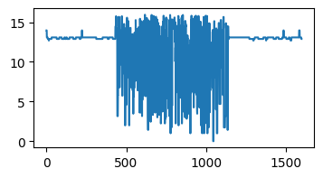
That doesn’t look right…
print(data.dtype)
uint8
Overflow#
The datatype uint8 only stores numbers between 0 and 255.
print(np.iinfo(data.dtype))
Machine parameters for uint8
---------------------------------------------------------------
min = 0
max = 255
---------------------------------------------------------------
By converting the dtype prior to the transformation to intensity, we make sure that we do not get any overflow.
data = np.asarray(im, dtype=np.int32)

line_pixels = data[:][ny // 2]

intensity = (
    line_pixels[:, 0] ** 2 + line_pixels[:, 1] ** 2 + line_pixels[:, 2] ** 2
) ** 0.5
plt.plot(intensity)
print(np.iinfo(data.dtype))
Machine parameters for int32
---------------------------------------------------------------
min = -2147483648
max = 2147483647
---------------------------------------------------------------

More constructions of numpy arrays#
Python lists and numpy arrays#
From list to array#
array(list, [datatype]) generates a numpy.array from a list:
mylist = [0, 1.2, 4, -9.1, 5, 8]

a = np.array(mylist)
From array to list#
a.tolist()
[0.0, 1.2, 4.0, -9.1, 5.0, 8.0]
From “anything” to NumPy array#
asarray(a)
converts “any” object a to a NumPy array if possible/necessary, tries to avoid copying.
Works with int’s, list’s, tuple’s, numpy.array’s, pil images, …
im = Image.open("figs/blackhole.jpg")

data = np.asarray(im)
print(data[:2][:2])
[[[11  5  5]
  [11  5  5]
  [11  5  5]
  ...
  [11  5  5]
  [11  5  5]
  [11  5  5]]

 [[11  5  5]
  [11  5  5]
  [11  5  5]
  ...
  [11  5  5]
  [11  5  5]
  [11  5  5]]]
Another example: Use asarray to allow flexible arguments in functions:
lst = [1, 2, 3]  # list
a = np.zeros(4)  # array
fl = -4.5  # float


def myfunc(some_sequence):
    a = np.asarray(some_sequence)
    return 3 * a - 5


for input_item in (lst, a, fl):
    print(f"Input: {input_item}, type:{type(input_item)}")
    print(f"Output:  3 * a - 5 ={ myfunc(input_item) } \n")
Input: [1, 2, 3], type:<class 'list'>
Output:  3 * a - 5 =[-2  1  4]

Input: [0. 0. 0. 0.], type:<class 'numpy.ndarray'>
Output:  3 * a - 5 =[-5. -5. -5. -5.]

Input: -4.5, type:<class 'float'>
Output:  3 * a - 5 =-18.5
Exercise: What would happen if we did not use a = np.asarray(some_sequence) inside myfunc?
Higher-dimensional arrays#
Passing a tuple to an array constructor results in a higher-dimensional array:
np.zeros((2, 2, 3)) # 2*3*3 dim. array
array([[[0., 0., 0.],
        [0., 0., 0.]],

       [[0., 0., 0.],
        [0., 0., 0.]]])
A two-dimensional array from two one-dimensional Python lists:
x = [0, 0.5, 1]
y = [-6.1, -2, 1.2]  # Python lists
np.array([x, y])  # form array with x and y as rows
array([[ 0. ,  0.5,  1. ],
       [-6.1, -2. ,  1.2]])
Numpy allows up to 32 dimensions. You can retrieve the shape of an array with
a = np.zeros((2, 3, 3))
a.shape
(2, 3, 3)
Changing array dimensions#
Use reshape to reinterpret the same data as a new shape without copying data:
a = np.array([0, 1.2, 4, -9.1, 5, 2])
b = a.reshape((2, 3))  # turn a into a 2x3 matrix
b
array([[10. ,  1.2,  4. ],
       [-9.1,  5. ,  2. ]])
Array view#
The reshaped array points to the same data vector, i.e. no data is copied:
b[0, 0]
0.0
b[0, 0] = -10
print(f"a = {a}")
print(f"b = \n{b}")
a = [-10.    1.2   4.   -9.1   5.    2. ]
b =
[[-10.    1.2   4. ]
 [ -9.1   5.    2. ]]
NumPy data ordering#
Numpy allows to store array in C or FORTRAN ordering:
 **Note**: For one-dimensional arrays, the orders are equivalent.
The order can be chosen with the order flag:
a = np.asarray([[1, 2], [3, 4]], order="F")  # Fortran order
a.flags.f_contiguous  # Check if Fortran ordering is used
True
NumPy data ordering (2)#
Numpy automatically converts the ordering when necessary:
A = np.array([[1, 2], [3, 4]], order="C")
B = np.array([[1, 2], [3, 4]], order="F")
print(A + B)
[[2 4]
 [6 8]]
Transposing a matrix is perfomed by swapping the ordering (without data copying):
A.transpose().flags.f_contiguous
True
Array indexing#
The indexing syntax that we are know from lists also work for arrays.
Getting values#
Slicing:
a[1:4] # Get 2nd to 4th element
Fancy indexing:
a[[0, 2, 3]] # Get entries 0, 2 and 3
Important: Slicing returns a view to the original array, i.e. no data is copied. Fancy indexing always returns a copy of the array.
Setting values#
a[2:4] = -1      # set a[2] and a[3] equal to -1
a[-1]  = a[0]    # set last equal to first element
a[:]   = 0       # set all elements of a equal to 0
Multi-dimensional indexing#
Multi-dimensional indexing has the same syntax as with list’s:
a = ones([2, 3]) # create a 2x3 matrix
                 # (two rows, three columns)

a[1,2] = 10      # set element (1,2) (2nd row, 3rd column)
a[1][2] = 10     # equivalent syntax (slower)
a[:,2] = 10      # set all elements in 3rd column
a[1,:] = 10      # set all elements in 2nd row
a[:,:] = 10       # set all elements
Example: extracting sub-matrices with slicing#
Given this matrix:
a = np.linspace(1, 2, 12).reshape(3, 4)
print(a)
[[1.         1.09090909 1.18181818 1.27272727]
 [1.36363636 1.45454545 1.54545455 1.63636364]
 [1.72727273 1.81818182 1.90909091 2.        ]]
we can use slicing to get a view of a subset of this matrix. For example to get the submatrix consisting of row 2 and 3 and every second column, we could use:
a[1:3, ::2] = 0  # a[i,j] for i=1,2 and j=0,2,4
a
array([[1.        , 1.09090909, 1.18181818, 1.27272727],
       [0.        , 1.45454545, 0.        , 1.63636364],
       [0.        , 1.81818182, 0.        , 2.        ]])
Slices create views of array data#
Assigning to a sliced array will change the original array:
a = np.ones([3, 2])
b = a[2, :]  # get a view onto the 3rd row
b[0] = np.pi  # assigning to b is reflected in a!
print(a)
[[1.         1.        ]
 [1.         1.        ]
 [3.14159265 1.        ]]
To avoid referencing via slices (if needed) use copy:
b = a[2,:].copy() # b has its own vector structure
Note: This behaviour is different to Python lists, where a[:] makes always a copy
Loops#
Loops over arrays using indices#
If we know the dimension of the array, we can use a nested loop to iterate over all array elements:
for i in range(a.shape[0]):
    for j in range(a.shape[1]):
        a[i, j] = (i + 1) * (j + 1) * (j + 2)
        print(f"a[{i}, {j}] = {a[i, j]}")
    print()  # empty line after each row
a[0, 0] = 2.0
a[0, 1] = 6.0

a[1, 0] = 4.0
a[1, 1] = 12.0

a[2, 0] = 6.0
a[2, 1] = 18.0
Is there a more Pythonic way?
What if we do not know the dimension of the array?
Better: Use standard Python loops#
A standard for loop iterates over the first index.
Example: Looping over each element in a matrix:
for row in a:
    for element in row:
         my_func(element)
For unknown dimensions loop over the flattened array#
View array as one-dimensional and iterate over all elements:
for element in a.ravel():
    my_func(element)
ravel() returns a flattened array, (1D version). Might return a copy if necessary.
Advice: Use ravel() only when reading elements, for assigning it is better to use shape or reshape.
Numpy Array computations#
Arithmetic operations#
Arithmetic operations can be used with arrays:
import numpy as np

a = np.linspace(0, 10, 11)

b = 3 * a - 1
c = np.sin(b)
d = np.exp(c)

print(b)
[-1. 2. 5. 8. 11. 14. 17. 20. 23. 26. 29.]
Note: most arithmetic operations in numpy are performed elementwise.
Array operations are much faster than element-wise operations#
Let’s compare the array versus element-wise operation on a 10 million large array.
Element-wise implementation#
%%time
import numpy as np

a = np.linspace(0, 1, int(1e07))  # create a large array

b = np.empty_like(a)
for i in range(a.size):
    b[i] = 3 * a[i] - 1
CPU times: user 1.68 s, sys: 17.5 ms, total: 1.7 s
Wall time: 1.69 s
Implementation with array operations#
%time b = 3 * a - 1
CPU times: user 10.2 ms, sys: 13.1 ms, total: 23.3 ms
Wall time: 21.9 ms
Array operators are typically faster as they are vectorized.
Vectorization of user-defined functions#
Imagine you have implemented your own function and would like to apply it to all elements in an array:
a = np.linspace(-1, 1, 10_000_000).reshape(10_000_000 // 2, 2)


def myfunc(x):
    if x > 0:
        return 0
    else:
        return x**2


myfunc(a)  # ??
---------------------------------------------------------------------------
ValueError                                Traceback (most recent call last)
Cell In [82], line 11
      7     else:
      8         return x**2
---> 11 myfunc(a)  # ??

Cell In [82], line 5, in myfunc(x)
      4 def myfunc(x):
----> 5     if x > 0:
      6         return 0
      7     else:

ValueError: The truth value of an array with more than one element is ambiguous. Use a.any() or a.all()
Problem: myfunc operates on the entire array instead of elementwise operations.
Potential solution to vectorization user-defined functions#
Loop over each array element and call myfunc
%%time
out = np.empty_like(a)
for i, ele in np.ndenumerate(a):
    out[i] = myfunc(ele)
CPU times: user 3.06 s, sys: 16.1 ms, total: 3.07 s
Wall time: 3.08 s
This is slow!
Better solution#
Convert myfunc to a vectorized function:
%%time
vfunc = np.vectorize(myfunc)
out2 = vfunc(a)
CPU times: user 775 ms, sys: 192 ms, total: 967 ms
Wall time: 966 ms
That’s faster!
Plotting with matplotlib#
Matplotlib is a popular package for creating publication quality figures. The easiest way to use matplotlib is to import the submodule “pyplot”.
Learning resources#
Matplotlib tutorial by Nicolas P. Rougier

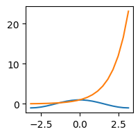
A simple plot#
Plotting one, or multiple sets of data is done with:
import matplotlib.pyplot as plt
import numpy as np

X = np.linspace(-np.pi, np.pi, 20, endpoint=True)
Y = np.cos(X)
Z = np.exp(X)

plt.figure(figsize=(2, 2))

plt.plot(X, Y)
plt.plot(X, Z)
[<matplotlib.lines.Line2D at 0x7fd3f5ea6500>]
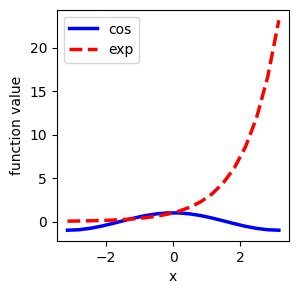
Adjusting your plot#
Typical adjustments:
Change line color, thickness, type
Change axis settings
Add labels, legends
…
plt.figure(figsize=(3, 3))
plt.plot(
    X, Y, label="cos", color="blue", linewidth=2.5, linestyle="-"
)  # Add labels for the legend
plt.plot(X, Z, label="exp", color="red", linewidth=2.5, linestyle="--")

plt.xlabel("x")  # Add labels for the axis
plt.ylabel("function value")  # Add labels for the axis

plt.legend(loc=0)
plt.savefig("file.pdf")  # save to files for use in papers, etc.
Other types of plots#
Function name |
Plot type |
|---|---|
pyplot.scatter |
Scatter plot |
pyplot.bar |
Bar plot |
pyplot.counturf |
Contour plot |
pyplot.imshow |
Showing images (on grids) |
pyplot.pie |
Pie charts |
pyplot.plot_surface |
3D charts |
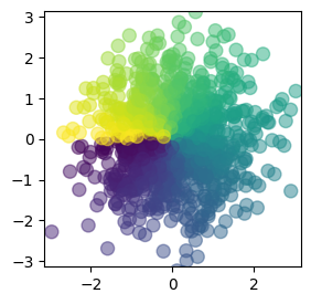
Example of a scatter plot#
n = 1024
X = np.random.normal(0, 1, n)
Y = np.random.normal(0, 1, n)
T = np.arctan2(Y, X)

plt.figure(figsize=(3, 3))
plt.scatter(X, Y, s=75, c=T, alpha=0.5)
plt.xlim([-np.pi, np.pi])
plt.ylim([-np.pi, np.pi])
(-3.141592653589793, 3.141592653589793)
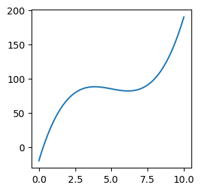
Plotting a function of x#
To start trying out plotting, let’s first define a function to plot: $\( f(x) = (x - 3) (x - 5) (x - 7) + 85 \)$
def func(x):
    return (x - 3) * (x - 5) * (x - 7) + 85
Next, we plot this function on \( \ x \in [0, 10] \)
# Calculate plot points:
x = np.linspace(0, 10)

# Evaluate the function at the plot points
y = func(x)

# Plot graph defined by x/y points
plt.figure(figsize=(3, 3))
plt.plot(x, y)
[<matplotlib.lines.Line2D at 0x7fd3fe1649a0>]