What is pandas good for?#
Working with (large) data sets and created automated data processes.
Pandas is extensively used to prepare data in data science (machine learning, data analytics, …)
Examples:
Import and export data into standard formats (CSV, Excel, Latex, ..).
Combine with Numpy for advanced computations or Matplotlib for visualisations.
Calculate statistics and answer questions about the data, like
What’s the average, median, max, or min of each column?
Does column A correlate with column B?
What does the distribution of data in column C look like?
Clean up data (e.g. fill out missing information and fix inconsistent formatting) and merge multiple data sets into one common dataset.
import pandas as pd
import pylab as pl
First, a short recap of the video session
The two fundamental data-structures in pandas are Series and DataFrame:
s = pd.Series([1, 2, 3])
s
0    1
1    2
2    3
dtype: int64
s = pd.Series([1, 2, 3], index=["a", "b", "c"])
s
a    1
b    2
c    3
dtype: int64
dic = {"a": 1, "b": 2, "c": 3}
s = pd.Series(dic)
s
a    1
b    2
c    3
dtype: int64
s["a"]
1
dic = {"a": [1, 2], "b": [3, 4], "c": [5, 6]}
s = pd.DataFrame(dic)
s
| a | b | c | |
|---|---|---|---|
| 0 | 1 | 3 | 5 |
| 1 | 2 | 4 | 6 |
s["a"]
0    1
1    2
Name: a, dtype: int64
s["a"][0]
1
s.columns
Index(['a', 'b', 'c'], dtype='object')
Reading data from file#
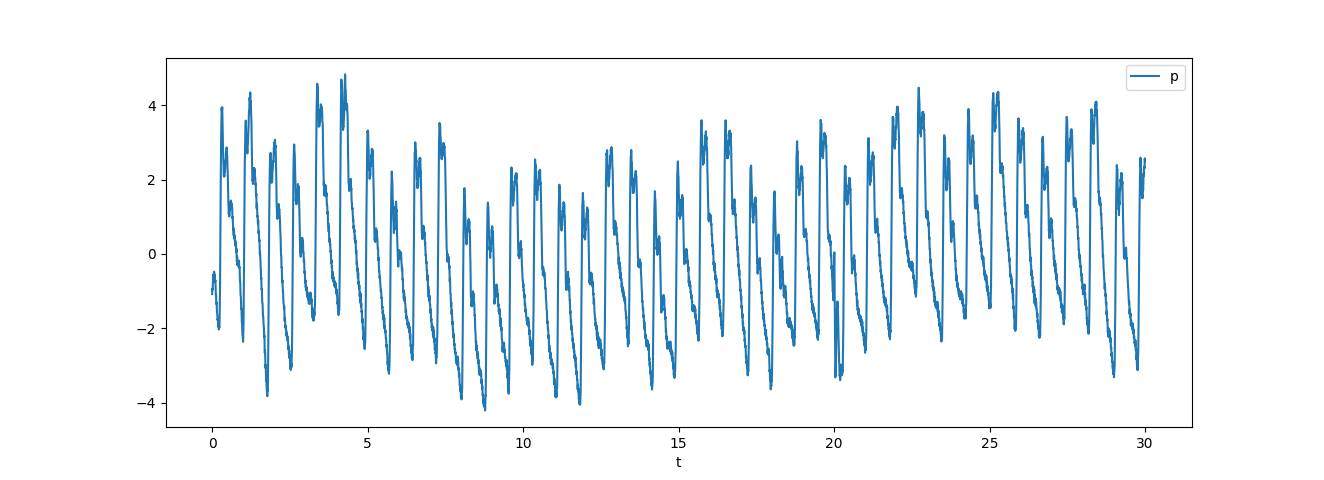
Now assume that we have some pressure data obtained from a sensor, as shown below
df = pd.read_csv("data/pressure.csv")
df
| Unnamed: 0 | t | p | |
|---|---|---|---|
| 0 | 0 | 0.000 | -1.077684 |
| 1 | 1 | 0.005 | -0.933488 |
| 2 | 2 | 0.010 | -0.956377 |
| 3 | 3 | 0.015 | -0.963243 |
| 4 | 4 | 0.020 | -0.864824 |
| ... | ... | ... | ... |
| 5995 | 5995 | 29.975 | 2.296034 |
| 5996 | 5996 | 29.980 | 2.312056 |
| 5997 | 5997 | 29.985 | 2.488295 |
| 5998 | 5998 | 29.990 | 2.570692 |
| 5999 | 5999 | 29.995 | 2.472273 |
6000 rows × 3 columns
t = df["t"]
p = df["p"]
p
0      -1.077684
1      -0.933488
2      -0.956377
3      -0.963243
4      -0.864824
          ...
5995    2.296034
5996    2.312056
5997    2.488295
5998    2.570692
5999    2.472273
Name: p, Length: 6000, dtype: float64
pl.plot(t, p)
pl.show()
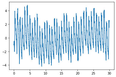
This way of extracting data from the DataFrame is useful for futher computations with t and p. For plotting purposes only, the DataFrame has its own plot-function:
df.plot()
pl.show()

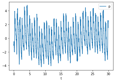
df.plot("t", "p")
pl.show()
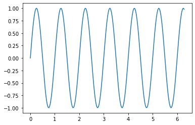
How to write data to csv#
t = pl.linspace(0, 2 * pl.pi, 200)
p = pl.sin(2 * pl.pi * t)
pl.plot(t, p)
pl.show()
data = pl.array([t, p])
When dealing with table data, you should always consider whether to use the .transpose() of a matrix
df = pd.DataFrame(data.transpose(), columns=["t", "p"])
df
| t | p | |
|---|---|---|
| 0 | 0.000000 | 0.000000 |
| 1 | 0.031574 | 0.197085 |
| 2 | 0.063148 | 0.386439 |
| 3 | 0.094721 | 0.560635 |
| 4 | 0.126295 | 0.712838 |
| ... | ... | ... |
| 195 | 6.156890 | 0.833697 |
| 196 | 6.188464 | 0.926180 |
| 197 | 6.220038 | 0.982332 |
| 198 | 6.251612 | 0.999949 |
| 199 | 6.283185 | 0.978341 |
200 rows × 2 columns
df.to_csv("pressure_computed.csv")
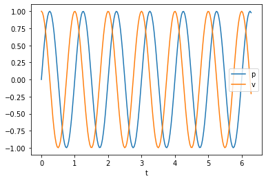
Adding a column to the existing DataFrame:#
v = pl.cos(2 * pl.pi * t)
v
array([ 1.        ,  0.98038635,  0.92231478,  0.82806328,  0.70132909,
        0.54708365,  0.37137759,  0.18110338, -0.01627502, -0.213015  ,
       -0.40139897, -0.57403714, -0.72415738, -0.84587087, -0.93440313,
       -0.98628127, -0.99947025, -0.9734527 , -0.90924922, -0.80937835,
       -0.67775774, -0.51955052, -0.34096273, -0.14899989,  0.04880781,
        0.24470092,  0.43099506,  0.60038243,  0.74621842,  0.86278226,
        0.94550148,  0.99113122,  0.99788155,  0.96548768,  0.89522032,
        0.78983588,  0.6534683 ,  0.49146692,  0.31018662,  0.11673853,
       -0.0812889 , -0.27612758, -0.46013452, -0.62609162, -0.76748884,
       -0.87877953, -0.95559807, -0.99493106, -0.99523559, -0.95649971,
       -0.88024292, -0.76945657, -0.62848651, -0.46286261, -0.27908187,
       -0.08435349,  0.11368385,  0.30726168,  0.48878646,  0.65113746,
        0.7879461 ,  0.89384572,  0.96468219,  0.99767677,  0.99153518,
        0.94649833,  0.8643329 ,  0.74826202,  0.60283883,  0.4337679 ,
        0.24768142,  0.05187907, -0.14595836, -0.33807024, -0.51692053,
       -0.67549342, -0.80756852, -0.90796489, -0.97274423, -0.99936544,
       -0.98678423, -0.93549413, -0.84750712, -0.72627468, -0.57655245,
       -0.40421361, -0.21601856, -0.01934969,  0.17807823,  0.36852061,
        0.54450692,  0.69913369,  0.82633533,  0.92112205,  0.97977564,
        0.99999527,  0.98098778,  0.92349877,  0.8297834 ,  0.70351786,
        0.5496552 ,  0.37423105,  0.18412683, -0.0132002 , -0.21000942,
       -0.39858053, -0.5715164 , -0.72203322, -0.84422662, -0.93330329,
       -0.98576898, -0.9995656 , -0.97415196, -0.91052496, -0.81118052,
       -0.68001565, -0.52217559, -0.34385199, -0.15204001,  0.0457361 ,
        0.2417181 ,  0.42821815,  0.59792036,  0.74416776,  0.86122346,
        0.94449569,  0.99071789,  0.99807689,  0.96628403,  0.89658645,
        0.79171819,  0.65579296,  0.49414274,  0.31310862,  0.1197921 ,
       -0.07822354, -0.27317068, -0.45740207, -0.62369081, -0.76551384,
       -0.87730783, -0.95468738, -0.99461712, -0.99553071, -0.95739231,
       -0.88169799, -0.77141703, -0.63087545, -0.46558633, -0.28203351,
       -0.08741728,  0.1106281 ,  0.30433384,  0.48610138,  0.64880047,
        0.78604886,  0.89246268,  0.96386758,  0.99746256,  0.99192976,
        0.94748624,  0.86587537,  0.75029855,  0.60528953,  0.43653664,
        0.25065959,  0.05494983, -0.14291545, -0.33517455, -0.51428565,
       -0.67322271, -0.80575106, -0.90667196, -0.97202656, -0.99925118,
       -0.98727786, -0.93657629, -0.84913535, -0.72838512, -0.5790623 ,
       -0.40702443, -0.21902008, -0.02242417,  0.17505139,  0.36566015,
        0.54192504,  0.69693168,  0.82459956,  0.91992062,  0.97915568,
        0.99998109,  0.98157993,  0.92467404,  0.83149567,  0.70569997,
        0.55222156,  0.37708098,  0.18714853, -0.01012525, -0.20700185])
df["v"] = v
df
| t | p | v | |
|---|---|---|---|
| 0 | 0.000000 | 0.000000 | 1.000000 |
| 1 | 0.031574 | 0.197085 | 0.980386 |
| 2 | 0.063148 | 0.386439 | 0.922315 |
| 3 | 0.094721 | 0.560635 | 0.828063 |
| 4 | 0.126295 | 0.712838 | 0.701329 |
| ... | ... | ... | ... |
| 195 | 6.156890 | 0.833697 | 0.552222 |
| 196 | 6.188464 | 0.926180 | 0.377081 |
| 197 | 6.220038 | 0.982332 | 0.187149 |
| 198 | 6.251612 | 0.999949 | -0.010125 |
| 199 | 6.283185 | 0.978341 | -0.207002 |
200 rows × 3 columns
It is possible to create an empty DataFrame and just add the columns whenever you like:
empty_df = pd.DataFrame()
empty_df["t"] = t
empty_df["p"] = p
empty_df["v"] = v
empty_df
| t | p | v | |
|---|---|---|---|
| 0 | 0.000000 | 0.000000 | 1.000000 |
| 1 | 0.031574 | 0.197085 | 0.980386 |
| 2 | 0.063148 | 0.386439 | 0.922315 |
| 3 | 0.094721 | 0.560635 | 0.828063 |
| 4 | 0.126295 | 0.712838 | 0.701329 |
| ... | ... | ... | ... |
| 195 | 6.156890 | 0.833697 | 0.552222 |
| 196 | 6.188464 | 0.926180 | 0.377081 |
| 197 | 6.220038 | 0.982332 | 0.187149 |
| 198 | 6.251612 | 0.999949 | -0.010125 |
| 199 | 6.283185 | 0.978341 | -0.207002 |
200 rows × 3 columns
empty_df.plot("t", ["p", "v"]) # pl.plot(t,p,t,v) in matplotlib
<AxesSubplot:xlabel='t'>
Exercise
Create uniformly sampled time points between 0 and 30.
Generate positional data in the xy-plane given by [0.4*t + cos(t), sin(t)]
Create a DataFrame consisting of the three columns t, x and y
plot x versus y using first the matplotlib plot function and then the DataFrame plot-method
Velocity-data can be computed by \(v_{x_i} = \frac{x_{i+1} - x_i}{t_{i+1} - t_i}\), \(v_{y_i} = \frac{y_{i+1} - y_i}{t_{i+1} - t_i}\) 5. Compute the velocity data for x and y and add those as columns in the DataFrame
A real world example. Oslo bysykkel data#
We go to https://oslobysykkel.no/apne-data/historisk (you can also get there by “oslo bysykkel data historisk” on google). We download the September data as CSV.
import zipfile
from pathlib import Path

import requests


def download_file(filename, url):
    path = Path(filename)
    if path.exists():
        return path
    print(f"Downloading {path}")
    with requests.get(url, stream=True) as r:
        r.raise_for_status()
        with path.open("wb") as f:
            for chunk in r.iter_content(chunk_size=8192):
                f.write(chunk)
    return path


def download_trips(year, month):
    dest = Path("data") / f"oslo_bike_{year}_{month:02}.csv"
    return download_file(
        dest,
        f"https://data.urbansharing.com/oslobysykkel.no/trips/v1/{year}/{month:02}.csv",
    )


trip_csv = download_trips(2021, 9)
import pandas as pd
import pylab as pl

trips = pd.read_csv(trip_csv)
trips
| started_at | ended_at | duration | start_station_id | start_station_name | start_station_description | start_station_latitude | start_station_longitude | end_station_id | end_station_name | end_station_description | end_station_latitude | end_station_longitude | |
|---|---|---|---|---|---|---|---|---|---|---|---|---|---|
| 0 | 2021-09-01 03:00:15.478000+00:00 | 2021-09-01 03:20:12.685000+00:00 | 1197 | 620 | Bislettgata | ved Sofies Gate | 59.923774 | 10.734713 | 735 | Oslo Hospital | ved trikkestoppet | 59.903213 | 10.767344 |
| 1 | 2021-09-01 03:03:04.080000+00:00 | 2021-09-01 03:06:10.732000+00:00 | 186 | 422 | St. Hanshaugen | langs Waldemar Thranes gate | 59.923703 | 10.740542 | 499 | Bjerregaards gate | ovenfor Fredrikke Qvams gate | 59.925488 | 10.746058 |
| 2 | 2021-09-01 03:16:41.288000+00:00 | 2021-09-01 03:25:20.740000+00:00 | 519 | 424 | Birkelunden | langs Seilduksgata | 59.925611 | 10.760926 | 478 | Jernbanetorget | Europarådets plass | 59.911901 | 10.749929 |
| 3 | 2021-09-01 03:21:55.708000+00:00 | 2021-09-01 03:28:20.138000+00:00 | 384 | 446 | Bislett Stadion | ved rundkjøringen | 59.925471 | 10.731219 | 478 | Jernbanetorget | Europarådets plass | 59.911901 | 10.749929 |
| 4 | 2021-09-01 03:26:16.090000+00:00 | 2021-09-01 03:30:30.133000+00:00 | 254 | 514 | Sofienberggata | ved Sars gate | 59.921206 | 10.769989 | 542 | Grünerhagen Nord | ved Sofienberggata | 59.922426 | 10.755427 |
| ... | ... | ... | ... | ... | ... | ... | ... | ... | ... | ... | ... | ... | ... |
| 190000 | 2021-09-30 22:56:22.073000+00:00 | 2021-09-30 23:11:50.892000+00:00 | 928 | 415 | Sinsenveien | ved Kongehellegata | 59.929542 | 10.781053 | 537 | St. Olavs gate | ved Pilestredet | 59.917968 | 10.738629 |
| 190001 | 2021-09-30 22:57:17.478000+00:00 | 2021-09-30 23:01:52.188000+00:00 | 274 | 460 | Botanisk Hage sør | langs Jens Bjelkes gate | 59.915418 | 10.769330 | 475 | Hausmanns bru | langs Nylandsveien | 59.914651 | 10.759872 |
| 190002 | 2021-09-30 22:57:33.599000+00:00 | 2021-09-30 23:04:41.205000+00:00 | 427 | 399 | Uelands gate | Ved Ulvetrappen (Ilatrappen) | 59.929545 | 10.748986 | 622 | Pilestredet 63 | ved trikkestoppet | 59.923883 | 10.731363 |
| 190003 | 2021-09-30 22:58:05.623000+00:00 | 2021-09-30 23:05:39.679000+00:00 | 454 | 465 | Bjørvika | under broen Nylandsveien | 59.909006 | 10.756180 | 390 | Saga Kino | langs Olav Vs gate | 59.914240 | 10.732771 |
| 190004 | 2021-09-30 22:58:36.872000+00:00 | 2021-09-30 23:03:06.333000+00:00 | 269 | 412 | Jakob kirke | langs Torggata | 59.917866 | 10.754898 | 442 | Vulkan | ved Maridalsveien | 59.922510 | 10.751010 |
190005 rows × 13 columns
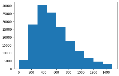
We can work with the data using normal pylab (and numpy functions):
pl.hist(trips["duration"], range=[0, 1500])
(array([ 5658., 28023., 40349., 35711., 26288., 17542., 11016.,  6854.,
         4433.,  2907.]),
 array([   0.,  150.,  300.,  450.,  600.,  750.,  900., 1050., 1200.,
        1350., 1500.]),
 <BarContainer object of 10 artists>)
We can also use DataFrame built-in functions:
trips.sort_values("duration")
| started_at | ended_at | duration | start_station_id | start_station_name | start_station_description | start_station_latitude | start_station_longitude | end_station_id | end_station_name | end_station_description | end_station_latitude | end_station_longitude | |
|---|---|---|---|---|---|---|---|---|---|---|---|---|---|
| 54120 | 2021-09-09 06:29:40.293000+00:00 | 2021-09-09 06:30:42.103000+00:00 | 61 | 381 | Grønlands torg | ved Tøyenbekken | 59.912520 | 10.762240 | 381 | Grønlands torg | ved Tøyenbekken | 59.912520 | 10.762240 |
| 150033 | 2021-09-23 16:57:04.305000+00:00 | 2021-09-23 16:58:05.488000+00:00 | 61 | 421 | Alexander Kiellands Plass | langs Maridalsveien | 59.928067 | 10.751203 | 421 | Alexander Kiellands Plass | langs Maridalsveien | 59.928067 | 10.751203 |
| 53582 | 2021-09-09 05:53:12.313000+00:00 | 2021-09-09 05:54:14.047000+00:00 | 61 | 623 | 7 Juni Plassen | langs Henrik Ibsens gate | 59.915060 | 10.731272 | 623 | 7 Juni Plassen | langs Henrik Ibsens gate | 59.915060 | 10.731272 |
| 70038 | 2021-09-11 09:08:26.043000+00:00 | 2021-09-11 09:09:27.337000+00:00 | 61 | 2304 | Hedmarksgata | ved Jordal Amfi | 59.911784 | 10.783884 | 2304 | Hedmarksgata | ved Jordal Amfi | 59.911784 | 10.783884 |
| 54483 | 2021-09-09 06:53:24.342000+00:00 | 2021-09-09 06:54:25.653000+00:00 | 61 | 474 | Blindern studentparkering | rett ved Blindern Studenterhjem | 59.940874 | 10.720779 | 474 | Blindern studentparkering | rett ved Blindern Studenterhjem | 59.940874 | 10.720779 |
| ... | ... | ... | ... | ... | ... | ... | ... | ... | ... | ... | ... | ... | ... |
| 52827 | 2021-09-08 21:45:08.196000+00:00 | 2021-09-09 05:06:05.736000+00:00 | 26457 | 1755 | Aker Brygge | ved trikkestopp | 59.911184 | 10.730035 | 1755 | Aker Brygge | ved trikkestopp | 59.911184 | 10.730035 |
| 92728 | 2021-09-14 22:37:30.359000+00:00 | 2021-09-15 06:03:14.857000+00:00 | 26744 | 525 | Myraløkka Øst | ved Bentsenbrua | 59.937205 | 10.760581 | 597 | Fredensborg | ved rundkjøringen | 59.920995 | 10.750358 |
| 94955 | 2021-09-15 07:51:00.736000+00:00 | 2021-09-15 15:25:43.368000+00:00 | 27282 | 468 | Skillebekk | langs Drammensveien | 59.912793 | 10.710103 | 390 | Saga Kino | langs Olav Vs gate | 59.914240 | 10.732771 |
| 8884 | 2021-09-02 07:15:39.199000+00:00 | 2021-09-02 15:05:55.621000+00:00 | 28216 | 615 | Munkedamsveien | ved Haakon VIIs gate | 59.913523 | 10.730106 | 580 | Georg Morgenstiernes hus | ved Moltke Moes vei | 59.939026 | 10.723003 |
| 125087 | 2021-09-20 06:48:08.055000+00:00 | 2021-09-20 16:12:09.094000+00:00 | 33841 | 506 | Botanisk Hage vest | ved Blytts gate | 59.920128 | 10.768875 | 569 | Botanisk hage sør-vest | ved Sars' gate | 59.917835 | 10.766374 |
190005 rows × 13 columns
trips["start_station_latitude"]
0         59.923774
1         59.923703
2         59.925611
3         59.925471
4         59.921206
            ...
190000    59.929542
190001    59.915418
190002    59.929545
190003    59.909006
190004    59.917866
Name: start_station_latitude, Length: 190005, dtype: float64
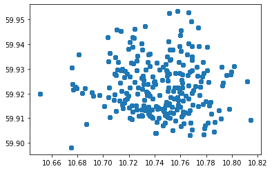
Exercise#
Make a scatter-plot showing the position (longitude, latitude) of stations in Oslo. It is OK to plot a station several times. Use matplotlib or the built-in DataFrame.plot.scatter
(Bonus) Make a scatter-plot with different size of the cirles, and let the size be dependent on how popular a station is (i.e. how many trips were started at the given station)
pl.scatter(trips["start_station_longitude"], trips["start_station_latitude"])
pl.show()
Let’s see if we can find information about how popular the different start stations are
trips["start_station_id"]
0         620
1         422
2         424
3         446
4         514
         ...
190000    415
190001    460
190002    399
190003    465
190004    412
Name: start_station_id, Length: 190005, dtype: int64
Let’s first try the numpy-way:
stations = pl.unique(trips["start_station_id"])
stations
array([ 377,  378,  380,  381,  382,  383,  384,  385,  387,  388,  389,
        390,  391,  392,  393,  394,  396,  397,  398,  399,  400,  401,
        402,  403,  404,  405,  406,  407,  408,  409,  410,  411,  412,
        413,  414,  415,  416,  417,  418,  420,  421,  422,  423,  424,
        425,  426,  427,  428,  429,  430,  431,  432,  433,  434,  435,
        436,  437,  438,  439,  440,  441,  442,  443,  444,  445,  446,
        447,  448,  449,  450,  451,  452,  453,  454,  455,  456,  457,
        458,  459,  460,  461,  462,  463,  464,  465,  466,  468,  469,
        470,  471,  472,  473,  474,  475,  476,  477,  478,  479,  480,
        481,  482,  483,  484,  486,  487,  488,  489,  491,  493,  494,
        495,  496,  497,  498,  499,  500,  501,  502,  503,  505,  506,
        507,  508,  509,  511,  512,  513,  514,  516,  518,  519,  521,
        522,  523,  524,  525,  526,  527,  529,  530,  531,  532,  533,
        534,  535,  536,  537,  540,  541,  542,  543,  545,  547,  548,
        549,  550,  551,  552,  553,  554,  555,  556,  557,  558,  559,
        560,  561,  562,  563,  564,  565,  567,  568,  569,  570,  572,
        573,  574,  575,  577,  578,  579,  580,  581,  582,  583,  584,
        585,  586,  587,  588,  589,  590,  591,  592,  593,  594,  595,
        596,  597,  598,  599,  600,  601,  602,  603,  605,  606,  607,
        608,  609,  610,  611,  612,  613,  614,  615,  616,  617,  618,
        619,  620,  621,  622,  623,  624,  625,  626,  627,  735,  737,
        738,  739,  742,  744,  746,  748,  787,  970, 1009, 1023, 1101,
       1755, 1919, 2270, 2280, 2304, 2305, 2306, 2307, 2308, 2309, 2315])
stations[0] == trips[
    "start_station_id"
]  # find out if trips started at the given station
0         False
1         False
2         False
3         False
4         False
          ...
190000    False
190001    False
190002    False
190003    False
190004    False
Name: start_station_id, Length: 190005, dtype: bool
(
    stations[0] == trips["start_station_id"]
).sum()  # sum all trips that started at the given station
680
Now we generalize the line above to create a list of number of trips for each station
number_of_trips = [
    (stations[i] == trips["start_station_id"]).sum() for i in range(len(stations))
]
number_of_trips
[680,
 562,
 1097,
 927,
 603,
 1115,
 1745,
 1450,
 585,
 628,
 400,
 1134,
 1431,
 606,
 822,
 994,
 1391,
 1592,
 2308,
 777,
 981,
 490,
 889,
 818,
 772,
 365,
 855,
 1020,
 2189,
 573,
 1004,
 724,
 1217,
 1548,
 684,
 316,
 578,
 674,
 427,
 950,
 2831,
 690,
 1278,
 1411,
 430,
 1050,
 597,
 285,
 376,
 629,
 813,
 417,
 613,
 855,
 814,
 838,
 936,
 1340,
 823,
 1355,
 217,
 1188,
 1495,
 1739,
 200,
 2038,
 1386,
 622,
 515,
 908,
 585,
 659,
 666,
 96,
 743,
 665,
 675,
 836,
 536,
 1572,
 369,
 1045,
 788,
 1606,
 1082,
 281,
 964,
 658,
 582,
 324,
 512,
 567,
 578,
 590,
 993,
 644,
 1632,
 1344,
 1947,
 454,
 243,
 548,
 765,
 588,
 784,
 703,
 1717,
 461,
 1437,
 677,
 671,
 755,
 565,
 211,
 1532,
 728,
 433,
 1046,
 1213,
 565,
 599,
 1257,
 380,
 313,
 1053,
 914,
 332,
 881,
 442,
 568,
 1086,
 1320,
 533,
 466,
 337,
 814,
 896,
 479,
 428,
 794,
 302,
 269,
 350,
 556,
 790,
 282,
 1179,
 769,
 377,
 848,
 582,
 323,
 418,
 508,
 904,
 197,
 2199,
 478,
 850,
 477,
 478,
 507,
 1356,
 837,
 494,
 74,
 716,
 835,
 785,
 1116,
 132,
 633,
 528,
 469,
 179,
 585,
 67,
 623,
 801,
 344,
 781,
 1339,
 1155,
 894,
 1440,
 851,
 630,
 628,
 622,
 634,
 168,
 355,
 1147,
 81,
 267,
 207,
 426,
 143,
 498,
 934,
 1487,
 493,
 719,
 179,
 159,
 1096,
 301,
 215,
 2132,
 680,
 477,
 563,
 826,
 467,
 480,
 797,
 349,
 298,
 769,
 617,
 547,
 2056,
 460,
 561,
 931,
 704,
 721,
 274,
 126,
 1026,
 1126,
 311,
 929,
 532,
 767,
 193,
 417,
 760,
 573,
 117,
 869,
 153,
 1203,
 88,
 331,
 403,
 425,
 576,
 170,
 604,
 342,
 214,
 838]
Now let’s try some pandas: For the only purpose of counting trips per station we may use .value_counts()
number_of_trips_pandas = trips["start_station_id"].value_counts()
number_of_trips_pandas
421     2831
398     2308
551     2199
408     2189
607     2132
        ...
454       96
1919      88
591       81
560       74
573       67
Name: start_station_id, Length: 253, dtype: int64
Now let’s say in our case we want all the information we can get about the start station, not only the number of trips. To group the data by start_station_id and count, while still extracting other relevant data for the start station we can use groupby()
station_data = trips.groupby(
    [
        "start_station_id",
        "start_station_name",
        "start_station_description",
        "start_station_latitude",
        "start_station_longitude",
    ]
).count()
station_data
| started_at | ended_at | duration | end_station_id | end_station_name | end_station_description | end_station_latitude | end_station_longitude | |||||
|---|---|---|---|---|---|---|---|---|---|---|---|---|
| start_station_id | start_station_name | start_station_description | start_station_latitude | start_station_longitude | ||||||||
| 377 | Tøyenparken | ved Caltexløkka | 59.915667 | 10.777566 | 680 | 680 | 680 | 680 | 680 | 680 | 680 | 680 |
| 378 | Colosseum Kino | langs Fridtjof Nansens vei | 59.929843 | 10.711285 | 562 | 562 | 562 | 562 | 562 | 562 | 562 | 562 |
| 380 | Bentsebrugata | rett over busstoppet | 59.939230 | 10.759170 | 1097 | 1097 | 1097 | 1097 | 1097 | 1097 | 1097 | 1097 |
| 381 | Grønlands torg | ved Tøyenbekken | 59.912520 | 10.762240 | 927 | 927 | 927 | 927 | 927 | 927 | 927 | 927 |
| 382 | Stensgata | ved trikkestoppet | 59.929586 | 10.732839 | 603 | 603 | 603 | 603 | 603 | 603 | 603 | 603 |
| ... | ... | ... | ... | ... | ... | ... | ... | ... | ... | ... | ... | ... |
| 2306 | Økern Portal | ved Dag Hammarskjölds vei | 59.930972 | 10.801830 | 170 | 170 | 170 | 170 | 170 | 170 | 170 | 170 |
| 2307 | Domus Athletica | ved Vestgrensa Studentby | 59.946219 | 10.724626 | 604 | 604 | 604 | 604 | 604 | 604 | 604 | 604 |
| 2308 | Gunerius | motsatt side av Torggata fra Gunerius bygget | 59.914638 | 10.753428 | 342 | 342 | 342 | 342 | 342 | 342 | 342 | 342 |
| 2309 | Ulven Torg | ved ulvenveien | 59.924960 | 10.812061 | 214 | 214 | 214 | 214 | 214 | 214 | 214 | 214 |
| 2315 | Rostockgata | ved Operagata | 59.906890 | 10.760307 | 838 | 838 | 838 | 838 | 838 | 838 | 838 | 838 |
254 rows × 8 columns
station_data = station_data.reset_index()
station_data
| start_station_id | start_station_name | start_station_description | start_station_latitude | start_station_longitude | started_at | ended_at | duration | end_station_id | end_station_name | end_station_description | end_station_latitude | end_station_longitude | |
|---|---|---|---|---|---|---|---|---|---|---|---|---|---|
| 0 | 377 | Tøyenparken | ved Caltexløkka | 59.915667 | 10.777566 | 680 | 680 | 680 | 680 | 680 | 680 | 680 | 680 |
| 1 | 378 | Colosseum Kino | langs Fridtjof Nansens vei | 59.929843 | 10.711285 | 562 | 562 | 562 | 562 | 562 | 562 | 562 | 562 |
| 2 | 380 | Bentsebrugata | rett over busstoppet | 59.939230 | 10.759170 | 1097 | 1097 | 1097 | 1097 | 1097 | 1097 | 1097 | 1097 |
| 3 | 381 | Grønlands torg | ved Tøyenbekken | 59.912520 | 10.762240 | 927 | 927 | 927 | 927 | 927 | 927 | 927 | 927 |
| 4 | 382 | Stensgata | ved trikkestoppet | 59.929586 | 10.732839 | 603 | 603 | 603 | 603 | 603 | 603 | 603 | 603 |
| ... | ... | ... | ... | ... | ... | ... | ... | ... | ... | ... | ... | ... | ... |
| 249 | 2306 | Økern Portal | ved Dag Hammarskjölds vei | 59.930972 | 10.801830 | 170 | 170 | 170 | 170 | 170 | 170 | 170 | 170 |
| 250 | 2307 | Domus Athletica | ved Vestgrensa Studentby | 59.946219 | 10.724626 | 604 | 604 | 604 | 604 | 604 | 604 | 604 | 604 |
| 251 | 2308 | Gunerius | motsatt side av Torggata fra Gunerius bygget | 59.914638 | 10.753428 | 342 | 342 | 342 | 342 | 342 | 342 | 342 | 342 |
| 252 | 2309 | Ulven Torg | ved ulvenveien | 59.924960 | 10.812061 | 214 | 214 | 214 | 214 | 214 | 214 | 214 | 214 |
| 253 | 2315 | Rostockgata | ved Operagata | 59.906890 | 10.760307 | 838 | 838 | 838 | 838 | 838 | 838 | 838 | 838 |
254 rows × 13 columns
station_data = station_data.drop(columns=station_data.columns[-7:])
station_data
| start_station_id | start_station_name | start_station_description | start_station_latitude | start_station_longitude | started_at | |
|---|---|---|---|---|---|---|
| 0 | 377 | Tøyenparken | ved Caltexløkka | 59.915667 | 10.777566 | 680 |
| 1 | 378 | Colosseum Kino | langs Fridtjof Nansens vei | 59.929843 | 10.711285 | 562 |
| 2 | 380 | Bentsebrugata | rett over busstoppet | 59.939230 | 10.759170 | 1097 |
| 3 | 381 | Grønlands torg | ved Tøyenbekken | 59.912520 | 10.762240 | 927 |
| 4 | 382 | Stensgata | ved trikkestoppet | 59.929586 | 10.732839 | 603 |
| ... | ... | ... | ... | ... | ... | ... |
| 249 | 2306 | Økern Portal | ved Dag Hammarskjölds vei | 59.930972 | 10.801830 | 170 |
| 250 | 2307 | Domus Athletica | ved Vestgrensa Studentby | 59.946219 | 10.724626 | 604 |
| 251 | 2308 | Gunerius | motsatt side av Torggata fra Gunerius bygget | 59.914638 | 10.753428 | 342 |
| 252 | 2309 | Ulven Torg | ved ulvenveien | 59.924960 | 10.812061 | 214 |
| 253 | 2315 | Rostockgata | ved Operagata | 59.906890 | 10.760307 | 838 |
254 rows × 6 columns
station_data = station_data.rename(columns={"started_at": "started_trips"})
station_data = station_data.set_index("start_station_id")
station_data
| start_station_name | start_station_description | start_station_latitude | start_station_longitude | started_trips | |
|---|---|---|---|---|---|
| start_station_id | |||||
| 377 | Tøyenparken | ved Caltexløkka | 59.915667 | 10.777566 | 680 |
| 378 | Colosseum Kino | langs Fridtjof Nansens vei | 59.929843 | 10.711285 | 562 |
| 380 | Bentsebrugata | rett over busstoppet | 59.939230 | 10.759170 | 1097 |
| 381 | Grønlands torg | ved Tøyenbekken | 59.912520 | 10.762240 | 927 |
| 382 | Stensgata | ved trikkestoppet | 59.929586 | 10.732839 | 603 |
| ... | ... | ... | ... | ... | ... |
| 2306 | Økern Portal | ved Dag Hammarskjölds vei | 59.930972 | 10.801830 | 170 |
| 2307 | Domus Athletica | ved Vestgrensa Studentby | 59.946219 | 10.724626 | 604 |
| 2308 | Gunerius | motsatt side av Torggata fra Gunerius bygget | 59.914638 | 10.753428 | 342 |
| 2309 | Ulven Torg | ved ulvenveien | 59.924960 | 10.812061 | 214 |
| 2315 | Rostockgata | ved Operagata | 59.906890 | 10.760307 | 838 |
254 rows × 5 columns
station_data.sort_values("started_trips", ascending=False)
| start_station_name | start_station_description | start_station_latitude | start_station_longitude | started_trips | |
|---|---|---|---|---|---|
| start_station_id | |||||
| 421 | Alexander Kiellands Plass | langs Maridalsveien | 59.928067 | 10.751203 | 2831 |
| 398 | Ringnes Park | ved Sannergata | 59.928434 | 10.759430 | 2308 |
| 551 | Olaf Ryes plass | langs Sofienberggata | 59.922425 | 10.758182 | 2198 |
| 408 | Tøyen skole | forsiden av skolebygget | 59.914943 | 10.773977 | 2189 |
| 607 | Marcus Thranes gate | ved Akerselva | 59.932772 | 10.758595 | 2132 |
| ... | ... | ... | ... | ... | ... |
| 454 | Furulund | langs Vækerøveien | 59.919810 | 10.651118 | 96 |
| 1919 | Kværnerveien | Ved Kværnerveien 5 | 59.905911 | 10.778592 | 88 |
| 591 | Grenseveien | ved Togbru | 59.924645 | 10.781727 | 81 |
| 560 | Gaustad T-bane | langs Slemdalsveien | 59.945955 | 10.710392 | 74 |
| 573 | Tordenskiolds gate | ved Rådhusgata | 59.911776 | 10.735113 | 67 |
254 rows × 5 columns
ended_trips = trips["end_station_id"].value_counts()
ended_trips
421     2818
551     2702
443     2676
489     2644
480     2479
        ...
591       80
1919      71
498       60
560       51
601       43
Name: end_station_id, Length: 253, dtype: int64
station_data["ended_trips"] = ended_trips
station_data.sort_values("started_trips", ascending=False)
| start_station_name | start_station_description | start_station_latitude | start_station_longitude | started_trips | ended_trips | |
|---|---|---|---|---|---|---|
| start_station_id | ||||||
| 421 | Alexander Kiellands Plass | langs Maridalsveien | 59.928067 | 10.751203 | 2831 | 2818 |
| 398 | Ringnes Park | ved Sannergata | 59.928434 | 10.759430 | 2308 | 2308 |
| 551 | Olaf Ryes plass | langs Sofienberggata | 59.922425 | 10.758182 | 2198 | 2702 |
| 408 | Tøyen skole | forsiden av skolebygget | 59.914943 | 10.773977 | 2189 | 2183 |
| 607 | Marcus Thranes gate | ved Akerselva | 59.932772 | 10.758595 | 2132 | 1607 |
| ... | ... | ... | ... | ... | ... | ... |
| 454 | Furulund | langs Vækerøveien | 59.919810 | 10.651118 | 96 | 85 |
| 1919 | Kværnerveien | Ved Kværnerveien 5 | 59.905911 | 10.778592 | 88 | 71 |
| 591 | Grenseveien | ved Togbru | 59.924645 | 10.781727 | 81 | 80 |
| 560 | Gaustad T-bane | langs Slemdalsveien | 59.945955 | 10.710392 | 74 | 51 |
| 573 | Tordenskiolds gate | ved Rådhusgata | 59.911776 | 10.735113 | 67 | 124 |
254 rows × 6 columns
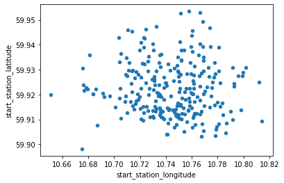
Plotting on a map with ipyleaflet and HTML#
We saw that the scatterplot could be used to plot stations on a map:
station_data.plot.scatter("start_station_longitude", "start_station_latitude")
<AxesSubplot:xlabel='start_station_longitude', ylabel='start_station_latitude'>
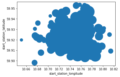
We now have tools to plot the most popular bike stations as bigger circles
station_data.plot.scatter(
    "start_station_longitude", "start_station_latitude", s="started_trips"
)
<AxesSubplot:xlabel='start_station_longitude', ylabel='start_station_latitude'>
ipywidgets/HTML and ipyleaflet are useful tools to visualize data on maps#
from ipyleaflet import Circle, Map, Marker, Polyline, basemap_to_tiles, basemaps
from ipywidgets import HTML
oslo_center = (
    59.9127,
    10.7461,
)  # NB ipyleaflet uses Lat-Long (i.e. y,x, when specifying coordinates)
oslo_map = Map(center=oslo_center, zoom=13)
oslo_map
oslo_map.save(
    "data/raw_oslo_map.html"
)  # if interactive view is not possible inline try to open this in your browser
We can add different layers to our map with a marker function. The function is written such that for a given row in the dataframe (i.e. a given station), we add one marker to the map
def add_markers(row):
    center = row["start_station_latitude"], row["start_station_longitude"]
    marker = Circle(
        location=center, radius=int(0.04 * row["started_trips"]), color="green"
    )
    oslo_map.add_layer(marker)
station_data.apply(add_markers, axis=1)
start_station_id
377     None
378     None
380     None
381     None
382     None
        ...
2306    None
2307    None
2308    None
2309    None
2315    None
Length: 254, dtype: object
Exercise#
Note: If you have issues with installing ipyleaflet or ipywidget with pip, just use pl.scatter() or pl.plot()
Create the DataFrame station_data as described in the lecture
Make a similar plot of the Oslo map with the most popular end-stations as red circles
Add the following line as the last line in your add_markers-function: marker.popup = HTML(f”{row[‘start_station_name’]} Trips started: {row[‘started_trips’]}”) . You can also add newlines within the string with the HTML command for newline
Try to make an Oslo map showing both started trips and ended trips in the same map
Make a map showing which stations are most popular going from Stensgata
ls data
FremontBridge.csv
bike-counter-locations-oslo-municipality.csv
car-counter-locations-oslo-municipality.csv
eustat_area.tsv
eustat_population.tsv
nor_population2022.csv
oslo_bike_2021_09.csv
oslo_bike_september_2022.csv
pressure.csv
pressure.png
raw_oslo_map.html
state-abbrevs.csv
state-areas.csv
state-population.csv
used_car_sales.csv
%reset
import pandas as pd
import pylab as pl

trip_csv = "data/oslo_bike_2021_09.csv"
trips = pd.read_csv(trip_csv)
station_data = trips.groupby(
    [
        "start_station_id",
        "start_station_longitude",
        "start_station_latitude",
        "start_station_name",
    ]
).count()
station_data = station_data.reset_index()
station_data = station_data.drop(columns=station_data.columns[-7:])
station_data = station_data.rename(columns={"started_at": "started_trips"})
station_data = station_data.set_index("start_station_id")
station_data["ended_trips"] = trips["end_station_id"].value_counts()

from ipyleaflet import Circle, Map, Marker, Polyline, basemap_to_tiles, basemaps
from ipywidgets import HTML

oslo_center = (
    59.9127,
    10.7461,
)  # NB ipyleaflet uses Lat-Long (i.e. y,x, when specifying coordinates)
oslo_map = Map(center=oslo_center, zoom=13)


def add_markers(row):
    center = row["start_station_latitude"], row["start_station_longitude"]
    marker = Circle(
        location=center, radius=int(0.04 * row["started_trips"]), color="green"
    )
    marker2 = Circle(
        location=center, radius=int(0.04 * row["ended_trips"]), color="red"
    )
    oslo_map.add_layer(marker)
    oslo_map.add_layer(marker2)
    marker.popup = HTML(
        f"{row['start_station_name']} <br> Trips started: {row['started_trips']}"
    )


station_data.apply(add_markers, axis=1)
oslo_map