Pandas - Data Analysis with Python

(last update 11/10/23)

Pandas is a high-performance, easy-to-use data structures and data analysis tools.

There is abundance of data and we should/need to make sense of it

• Smart devices, Strava, …

• SSB Statistics Norway *

• EuroStat Statistics Europe *

• Kaggle Data Science compatitions*

• Quandl for finances

• Yr

• Oslo Bysykkel API **

(We will work with these ones today in lecture* or exercises**)

What is Pandas good for?

Working with (large) data sets and created automated data processes.

Pandas is extensively used to prepare data in data science (machine learning, data analytics, …)

Examples:

• Import and export data into standard formats (CSV, Excel, Latex, ..).

• Combine with Numpy for advanced computations or Matplotlib for visualisations.

• Calculate statistics and answer questions about the data, like

• What’s the average, median, max, or min of each column?

  • Does column A correlate with column B?

  • What does the distribution of data in column C look like?

• Clean up data (e.g. fill out missing information and fix inconsistent formatting) and merge multiple data sets into one common one

More information

• Official Pandas documentation: http://pandas.pydata.org/pandas-docs/stable/tutorials.html

• Pandas cookbook: http://pandas.pydata.org/pandas-docs/stable/cookbook.html

• Wes McKinney, Python for Data Analysis

• Python Data Science Handbook by Jake VanderPlas (We follow Chapter 4 in this lecture)

This lecture

• Part1 Introduction to Pandas

• Part2 Hands on examples with real data

Installation

• If you have Anaconda: Already installed

• If you have Miniconda: conda install pandas

• If you have your another Python distribution: python3 -m pip install pandas

Let’s dive in

import pandas as pd

Pandas Series object

Series is 1d series of data similar to numpy.array.

series = pd.Series([4, 5, 6, 7, 8])
series.values

array([4, 5, 6, 7, 8])

series.index

RangeIndex(start=0, stop=5, step=1)

(series.values.dtype, series.index.dtype)

(dtype('int64'), dtype('int64'))

We see that series are indexed and both values and index are typed. As we saw with numpy this has performance benefits. The similarity with numpy.array

series[0]

4

import numpy as np

np.power(series, 2)

0    16
1    25
2    36
3    49
4    64
dtype: int64

However, the indices do not need to be numbers (and neither need to be the values)

values = list(range(65, 75))
index = [chr(v) for v in values]
series = pd.Series(values, index=index)
series

A    65
B    66
C    67
D    68
E    69
F    70
G    71
H    72
I    73
J    74
dtype: int64

The series than behaves also like a dictionary, although it supports fancy indexing.

series["A"], series["D":"H"]

(65,
 D    68
 E    69
 F    70
 G    71
 H    72
 dtype: int64)

Continuing the analogy with dictionary a possible way to make series is from a dictionary

data = {
    "Washington": "United States of America",
    "London": "Great Britain",
    "Oslo": "Norway",
}
series = pd.Series(data)
series

Washington    United States of America
London                   Great Britain
Oslo                            Norway
dtype: object

Note that for values that are amenable to str we have the string methods …

series.str.upper()

Washington    UNITED STATES OF AMERICA
London                   GREAT BRITAIN
Oslo                            NORWAY
dtype: object

… and so we can for example compute a mask using regular expressions (here looking for states with 2 word names) …

mask = series.str.match(r"^\w+\s+\w+$")
mask

Washington    False
London         True
Oslo          False
dtype: bool

… which can be used to index into the series

series[mask]

London    Great Britain
dtype: object

Some other examples of series indexing

(series[0], series["London":"Oslo"], series[0:2])

('United States of America',
 London    Great Britain
 Oslo             Norway
 dtype: object,
 Washington    United States of America
 London                   Great Britain
 dtype: object)

We can be more explicit about the indexing with indexers loc and iloc

(series.iloc[0], series.loc["London":"Oslo"], series.iloc[0:2])

('United States of America',
 London    Great Britain
 Oslo             Norway
 dtype: object,
 Washington    United States of America
 London                   Great Britain
 dtype: object)

series[1:3]

London    Great Britain
Oslo             Norway
dtype: object

import this

The Zen of Python, by Tim Peters

Beautiful is better than ugly.
Explicit is better than implicit.
Simple is better than complex.
Complex is better than complicated.
Flat is better than nested.
Sparse is better than dense.
Readability counts.
Special cases aren't special enough to break the rules.
Although practicality beats purity.
Errors should never pass silently.
Unless explicitly silenced.
In the face of ambiguity, refuse the temptation to guess.
There should be one-- and preferably only one --obvious way to do it.
Although that way may not be obvious at first unless you're Dutch.
Now is better than never.
Although never is often better than *right* now.
If the implementation is hard to explain, it's a bad idea.
If the implementation is easy to explain, it may be a good idea.
Namespaces are one honking great idea -- let's do more of those!

But why does this matter? Consider

tricky = pd.Series(["a", "b", "c"], index=[7, 5, 4])
tricky

7    a
5    b
4    c
dtype: object

# Let's demonstrate that we can sort
tricky = tricky.sort_index()

tricky

4    c
5    b
7    a
dtype: object

# Here we are refering to the value at row where index = 4 and values where at first though second row!
# Try tricky.loc[4] vs tricky.iloc[4]
(tricky.loc[4], tricky[0:2])

('c',
 4    c
 5    b
 dtype: object)

Pandas DataFrame object

Two dimensional data are represented by DataFrames. Again Pandas allows for flexibility of what row/columns indices can be. DataFrames can be constructed in a number of ways

def spreadsheet(nrows, ncols, start=0, cstart=0, base=0):
    data = base + np.random.rand(nrows, ncols)
    index = [f"r{i}" for i in range(start, start + nrows)]
    columns = [f"c{i}" for i in range(cstart, cstart + ncols)]
    # c0 c1 c2
    # r0
    # r1
    return pd.DataFrame(data, index=index, columns=columns)


data_frame = spreadsheet(10, 4)
data_frame["c0"]

r0    0.341584
r1    0.154689
r2    0.829218
r3    0.860563
r4    0.482496
r5    0.623338
r6    0.951465
r7    0.330926
r8    0.805647
r9    0.038046
Name: c0, dtype: float64

For large frame it is usefull to look at portions of the data

data_frame = spreadsheet(10_000, 4)
print(len(data_frame))
data_frame.head(10)  # data_frame.tail is for the end part

10000

	c0	c1	c2	c3
r0	0.658119	0.888360	0.151696	0.680974
r1	0.519551	0.838755	0.180593	0.933276
r2	0.149844	0.110505	0.253935	0.506687
r3	0.582279	0.171603	0.414131	0.822162
r4	0.721373	0.428403	0.404248	0.841991
r5	0.432620	0.953647	0.023574	0.614961
r6	0.939906	0.018228	0.556107	0.012206
r7	0.836547	0.463066	0.802324	0.835970
r8	0.440520	0.777486	0.042400	0.008710
r9	0.165533	0.267046	0.287619	0.101397

We can combines multiple series into a frame

index = ("Min", "Ingeborg", "Miro")
nationality = pd.Series(["USA", "NOR", "SVK"], index=index)
university = pd.Series(["Berkeley", "Bergen", "Oslo"], index=index)

instructors = pd.DataFrame({"nat": nationality, "uni": university})
instructors

	nat	uni
Min	USA	Berkeley
Ingeborg	NOR	Bergen
Miro	SVK	Oslo

(instructors.index, instructors.columns)

(Index(['Min', 'Ingeborg', 'Miro'], dtype='object'),
 Index(['nat', 'uni'], dtype='object'))

Anothor way of creating is using dictionaries

f = pd.DataFrame(
    {
        "country": ["CZE", "NOR", "USA"],
        "capital": ["Prague", "Oslo", "Washington DC"],
        "pop": [5, 10, 300],
    }
)
f

	country	capital	pop
0	CZE	Prague	5
1	NOR	Oslo	10
2	USA	Washington DC	300

When some column is unique we can designate it as index. Of course, tables can be stored in various formats. We will come back to reading later.

# LaTex
import re

fi = f.set_index("country")

tex_table = fi.style.to_latex()
# To ease the prining
for row in re.split(r"\n", tex_table):
    print(row)

\begin{tabular}{llr}
 & capital & pop \\
country &  &  \\
CZE & Prague & 5 \\
NOR & Oslo & 10 \\
USA & Washington DC & 300 \\
\end{tabular}

# CSV
tex_table = fi.to_csv(sep=";")
# To ease the prining
for row in re.split(r"\n", tex_table):
    print(row)

country;capital;pop
CZE;Prague;5
NOR;Oslo;10
USA;Washington DC;300

Going back to frame creation, recall that above, the two series had a common index. What happens with the frame when this is not the case? Below we also illustrate another constructor.

nationality = {"Miro": "SVK", "Ingeborg": "NOR", "Min": "USA"}
university = {"Miro": "Oslo", "Ingeborg": "Bergen", "Min": "Berkeley", "Joe": "Harvard"}
office = {"Miro": 303, "Ingeborg": 309, "Min": 311, "Joe": -1}
# Construct from list of dictionary using union of keys as columns - we need to fill in values for some
# NOTE: here each dictionary essentially defines a row
missing_data_frame = pd.DataFrame(
    [nationality, university, office], index=["nation", "uni", "office"]
)
missing_data_frame

	Miro	Ingeborg	Min	Joe
nation	SVK	NOR	USA	NaN
uni	Oslo	Bergen	Berkeley	Harvard
office	303	309	311	-1

# Just to make it look better
missing_data_frame = missing_data_frame.T
missing_data_frame

	nation	uni	office
Miro	SVK	Oslo	303
Ingeborg	NOR	Bergen	309
Min	USA	Berkeley	311
Joe	NaN	Harvard	-1

The missing value has been filled with a special value. Real data often suffer from lack of regularity. We can check for this

missing_data_frame.isna()

	nation	uni	office
Miro	False	False	False
Ingeborg	False	False	False
Min	False	False	False
Joe	True	False	False

And the provide a missing value. Note that this can be done already when we are constructing the frame.

missing_data_frame.fillna("OutThere")

	nation	uni	office
Miro	SVK	Oslo	303
Ingeborg	NOR	Bergen	309
Min	USA	Berkeley	311
Joe	OutThere	Harvard	-1

Or discard the data. We can drop the row which has NaN. Note that by default any NaN is enough but we can be more tolerant (see how and thresh keyword arguments)

missing_data_frame.dropna()

	nation	uni	office
Miro	SVK	Oslo	303
Ingeborg	NOR	Bergen	309
Min	USA	Berkeley	311

Or we drop the problematic column. Axis 0 is row (just like in numpy)

missing_data_frame.dropna(axis=1)

	uni	office
Miro	Oslo	303
Ingeborg	Bergen	309
Min	Berkeley	311
Joe	Harvard	-1

Note that the above calls are returning a new Frame, ie. are not in in-place. For this use .dropna(..., inplace=True)

Once we have the frame we can start computing with it. Let’s consider indexing first

missing_data_frame

	nation	uni	office
Miro	SVK	Oslo	303
Ingeborg	NOR	Bergen	309
Min	USA	Berkeley	311
Joe	NaN	Harvard	-1

# Get a specific series
missing_data_frame["nation"]

Miro        SVK
Ingeborg    NOR
Min         USA
Joe         NaN
Name: nation, dtype: object

# Or several as a frame
missing_data_frame[["nation", "uni"]]

	nation	uni
Miro	SVK	Oslo
Ingeborg	NOR	Bergen
Min	USA	Berkeley
Joe	NaN	Harvard

Note that slicing default to rows

# Will fail because no rows names like that
missing_data_frame["nation":"office"]

---------------------------------------------------------------------------
KeyError                                  Traceback (most recent call last)
File ~/.local/lib/python3.9/site-packages/pandas/core/indexes/base.py:3653, in Index.get_loc(self, key)
   3652 try:
-> 3653     return self._engine.get_loc(casted_key)
   3654 except KeyError as err:

File ~/.local/lib/python3.9/site-packages/pandas/_libs/index.pyx:147, in pandas._libs.index.IndexEngine.get_loc()

File ~/.local/lib/python3.9/site-packages/pandas/_libs/index.pyx:176, in pandas._libs.index.IndexEngine.get_loc()

File pandas/_libs/hashtable_class_helper.pxi:7080, in pandas._libs.hashtable.PyObjectHashTable.get_item()

File pandas/_libs/hashtable_class_helper.pxi:7088, in pandas._libs.hashtable.PyObjectHashTable.get_item()

KeyError: 'nation'

The above exception was the direct cause of the following exception:

KeyError                                  Traceback (most recent call last)
Cell In [37], line 2
      1 # Will fail because no rows names like that
----> 2 missing_data_frame["nation":"office"]

File ~/.local/lib/python3.9/site-packages/pandas/core/frame.py:3735, in DataFrame.__getitem__(self, key)
   3733 # Do we have a slicer (on rows)?
   3734 if isinstance(key, slice):
-> 3735     indexer = self.index._convert_slice_indexer(key, kind="getitem")
   3736     if isinstance(indexer, np.ndarray):
   3737         # reachable with DatetimeIndex
   3738         indexer = lib.maybe_indices_to_slice(
   3739             indexer.astype(np.intp, copy=False), len(self)
   3740         )

File ~/.local/lib/python3.9/site-packages/pandas/core/indexes/base.py:4132, in Index._convert_slice_indexer(self, key, kind)
   4130     indexer = key
   4131 else:
-> 4132     indexer = self.slice_indexer(start, stop, step)
   4134 return indexer

File ~/.local/lib/python3.9/site-packages/pandas/core/indexes/base.py:6344, in Index.slice_indexer(self, start, end, step)
   6300 def slice_indexer(
   6301     self,
   6302     start: Hashable | None = None,
   6303     end: Hashable | None = None,
   6304     step: int | None = None,
   6305 ) -> slice:
   6306     """
   6307     Compute the slice indexer for input labels and step.
   6308 
   (...)
   6342     slice(1, 3, None)
   6343     """
-> 6344     start_slice, end_slice = self.slice_locs(start, end, step=step)
   6346     # return a slice
   6347     if not is_scalar(start_slice):

File ~/.local/lib/python3.9/site-packages/pandas/core/indexes/base.py:6537, in Index.slice_locs(self, start, end, step)
   6535 start_slice = None
   6536 if start is not None:
-> 6537     start_slice = self.get_slice_bound(start, "left")
   6538 if start_slice is None:
   6539     start_slice = 0

File ~/.local/lib/python3.9/site-packages/pandas/core/indexes/base.py:6462, in Index.get_slice_bound(self, label, side)
   6459         return self._searchsorted_monotonic(label, side)
   6460     except ValueError:
   6461         # raise the original KeyError
-> 6462         raise err
   6464 if isinstance(slc, np.ndarray):
   6465     # get_loc may return a boolean array, which
   6466     # is OK as long as they are representable by a slice.
   6467     assert is_bool_dtype(slc.dtype)

File ~/.local/lib/python3.9/site-packages/pandas/core/indexes/base.py:6456, in Index.get_slice_bound(self, label, side)
   6454 # we need to look up the label
   6455 try:
-> 6456     slc = self.get_loc(label)
   6457 except KeyError as err:
   6458     try:

File ~/.local/lib/python3.9/site-packages/pandas/core/indexes/base.py:3655, in Index.get_loc(self, key)
   3653     return self._engine.get_loc(casted_key)
   3654 except KeyError as err:
-> 3655     raise KeyError(key) from err
   3656 except TypeError:
   3657     # If we have a listlike key, _check_indexing_error will raise
   3658     #  InvalidIndexError. Otherwise we fall through and re-raise
   3659     #  the TypeError.
   3660     self._check_indexing_error(key)

KeyError: 'nation'

# See that slice goes for rows
missing_data_frame["Miro":"Min"]

	nation	uni	office
Miro	SVK	Oslo	303
Ingeborg	NOR	Bergen	309
Min	USA	Berkeley	311

We can call indexers to rescue

missing_data_frame.loc[:, "nation":"uni"]

	nation	uni
Miro	SVK	Oslo
Ingeborg	NOR	Bergen
Min	USA	Berkeley
Joe	NaN	Harvard

Indexes can of course be more involed

missing_data_frame["office"] > 305

Miro        False
Ingeborg     True
Min          True
Joe         False
Name: office, dtype: bool

missing_data_frame.loc[missing_data_frame["office"] > 305, ["uni", "nation"]]

	uni	nation
Ingeborg	Bergen	NOR
Min	Berkeley	USA

Next let’s compute with the values in the frames

f0 = spreadsheet(4, 4)
np.cos(f0)

	c0	c1	c2	c3
r0	0.870461	0.789699	0.739024	0.860132
r1	0.785803	0.718719	0.580812	0.584109
r2	0.988713	0.956762	0.956623	0.851564
r3	0.559086	0.889881	0.990609	0.903777

Binary operation will align the frame - operation is valid only for the index-column pairs found in both and with will get missing for the rest

f1 = spreadsheet(5, 6)
f0 + f1

	c0	c1	c2	c3	c4	c5
r0	0.533858	0.997285	1.098653	1.032666	NaN	NaN
r1	1.372231	0.804163	1.445381	1.393992	NaN	NaN
r2	1.056678	0.809150	0.589316	0.936123	NaN	NaN
r3	1.311115	0.863243	0.404915	0.961394	NaN	NaN
r4	NaN	NaN	NaN	NaN	NaN	NaN

Note that this is note unique to frames and works (unsuprisingly on series too)

c00 = f0["c0"]
c10 = f1["c0"]
c00 + c10

r0    0.533858
r1    1.372231
r2    1.056678
r3    1.311115
r4         NaN
Name: c0, dtype: float64

Reduction operators default to be computed for each column

f1.max()

c0    0.906288
c1    0.514013
c2    0.883873
c3    0.519110
c4    0.910645
c5    0.811385
dtype: float64

For column wise reduction we need to specify the axis (axis=1)

f1.mean(axis="columns")

r0    0.339750
r1    0.554993
r2    0.498857
r3    0.482604
r4    0.406889
dtype: float64

Pandas Index object

In the previous usecase f0 + f1 we have seen that operation is performed for common keys - this suggests that we can do logical operations on indices. This is indeed the case

i0 = f0.index
i1 = f1.index
(i0.union(i1), i0.intersection(i1))

(Index(['r0', 'r1', 'r2', 'r3', 'r4'], dtype='object'),
 Index(['r0', 'r1', 'r2', 'r3'], dtype='object'))

Indexes can be explicitely constructed. For working with time series it is useful to index by time. Let’s get timestamp indexing for every Day between 2 dates

import datetime

time = pd.date_range(
    start=datetime.date.fromisoformat("2022-10-19"),
    end=datetime.date.fromisoformat("2022-12-20"),
    freq="D",
)
time

DatetimeIndex(['2022-10-19', '2022-10-20', '2022-10-21', '2022-10-22',
               '2022-10-23', '2022-10-24', '2022-10-25', '2022-10-26',
               '2022-10-27', '2022-10-28', '2022-10-29', '2022-10-30',
               '2022-10-31', '2022-11-01', '2022-11-02', '2022-11-03',
               '2022-11-04', '2022-11-05', '2022-11-06', '2022-11-07',
               '2022-11-08', '2022-11-09', '2022-11-10', '2022-11-11',
               '2022-11-12', '2022-11-13', '2022-11-14', '2022-11-15',
               '2022-11-16', '2022-11-17', '2022-11-18', '2022-11-19',
               '2022-11-20', '2022-11-21', '2022-11-22', '2022-11-23',
               '2022-11-24', '2022-11-25', '2022-11-26', '2022-11-27',
               '2022-11-28', '2022-11-29', '2022-11-30', '2022-12-01',
               '2022-12-02', '2022-12-03', '2022-12-04', '2022-12-05',
               '2022-12-06', '2022-12-07', '2022-12-08', '2022-12-09',
               '2022-12-10', '2022-12-11', '2022-12-12', '2022-12-13',
               '2022-12-14', '2022-12-15', '2022-12-16', '2022-12-17',
               '2022-12-18', '2022-12-19', '2022-12-20'],
              dtype='datetime64[ns]', freq='D')

We generate the corresponding data and illustrate some plotting capabilities of Pandas

import matplotlib.pyplot as plt

values = np.sin(np.pi / 10 * np.arange(len(time)))

time_series = pd.Series(values, index=time)
time_series.plot()

<AxesSubplot: >

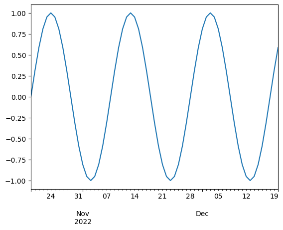
Note that we are getting the nice xlabels for free!

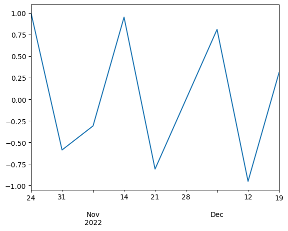
Time indexing allows us to do some fancy opearations. For example we can have a look at the signal for only the first day of the week (Monday?). For other functionality see resample, ‘rolling’ means on windows ets.

time_series[time.weekday == 0].plot()

<AxesSubplot: >

Note the value of difference between to time indices

time[:4] - time[1:5]

TimedeltaIndex(['-1 days', '-1 days', '-1 days', '-1 days'], dtype='timedelta64[ns]', freq=None)

The Timedelta object can be useful for shifting

diff = pd.Timedelta("1m")
time = time + diff
time[:5]

DatetimeIndex(['2022-10-19 00:01:00', '2022-10-20 00:01:00',
               '2022-10-21 00:01:00', '2022-10-22 00:01:00',
               '2022-10-23 00:01:00'],
              dtype='datetime64[ns]', freq='D')

Time stamps often come in different format. Pandas offers convenience functions for their conversion/parsing.

df = pd.DataFrame({"date": [1470195805, 1480195805, 1490195805], "value": [2, 3, 4]})
df

	date	value
0	1470195805	2
1	1480195805	3
2	1490195805	4

When was the clock started?

pd.to_datetime(df["date"], unit="s")

0   2016-08-03 03:43:25
1   2016-11-26 21:30:05
2   2017-03-22 15:16:45
Name: date, dtype: datetime64[ns]

import time

pd.to_datetime(pd.Series([0, time.time()]), unit="s")

0   1970-01-01 00:00:00.000000000
1   2023-10-12 07:10:21.943605760
dtype: datetime64[ns]

Question: how can we get the years prior to 1970 to work?

Hierarchical indexing with MultiIndex

Multiindexing is a way to handle higher order tensors, e.g. f(x, y, color). It also allows for organizing the data by establishing hierarchy in indexing. Suppose we have RGB image of 5 x 4 pixels. We could represent this as a table with channel x and y coordinate columns and 5 x 4 x 3 rows. A representation more true to the nature of the data would be to have a “column” for each color

column_index = pd.MultiIndex.from_product(
    [["R", "G", "B"], [0, 1, 2, 3]], names=("color", "cindex")
)
column_index

MultiIndex([('R', 0),
            ('R', 1),
            ('R', 2),
            ('R', 3),
            ('G', 0),
            ('G', 1),
            ('G', 2),
            ('G', 3),
            ('B', 0),
            ('B', 1),
            ('B', 2),
            ('B', 3)],
           names=['color', 'cindex'])

image = pd.DataFrame(
    np.arange(60).reshape(5, 12),
    index=pd.Index([0, 1, 2, 3, 4], name="rindex"),
    columns=column_index,
)
image

color	R				G				B
cindex	0	1	2	3	0	1	2	3	0	1	2	3
rindex
0	0	1	2	3	4	5	6	7	8	9	10	11
1	12	13	14	15	16	17	18	19	20	21	22	23
2	24	25	26	27	28	29	30	31	32	33	34	35
3	36	37	38	39	40	41	42	43	44	45	46	47
4	48	49	50	51	52	53	54	55	56	57	58	59

We can have a look at the said “flat” representation of the data

image.unstack()

color  cindex  rindex
R      0       0          0
               1         12
               2         24
               3         36
               4         48
       1       0          1
               1         13
               2         25
               3         37
               4         49
       2       0          2
               1         14
               2         26
               3         38
               4         50
       3       0          3
               1         15
               2         27
               3         39
               4         51
G      0       0          4
               1         16
               2         28
               3         40
               4         52
       1       0          5
               1         17
               2         29
               3         41
               4         53
       2       0          6
               1         18
               2         30
               3         42
               4         54
       3       0          7
               1         19
               2         31
               3         43
               4         55
B      0       0          8
               1         20
               2         32
               3         44
               4         56
       1       0          9
               1         21
               2         33
               3         45
               4         57
       2       0         10
               1         22
               2         34
               3         46
               4         58
       3       0         11
               1         23
               2         35
               3         47
               4         59
dtype: int64

Accessing the entries works as follows

image["R"]  # Column(s) where first multiindex is R
image.loc[:, ("R", 0)]  # Column multiindex by R, 0
image.loc[2, ("R", 1)]  # The entry

25

We can perform reduction operation

image.mean().mean()

29.5

Combining datasets - appending

Extend numpy.concatenate to pandas objects. We can combine data from 2 frames if they have some “axes” in common. Let’s start with 2 identical columns and do default vertical/row wise concatenation. Note that all the operations below create new DataFrame

# Unique row indices
d1 = spreadsheet(2, 2, base=0)
d2 = spreadsheet(4, 2, base=10)
print(d1)
print(d2)

          c0        c1
r0  0.904955  0.461721
r1  0.728287  0.227259
           c0         c1
r0  10.784765  10.696760
r1  10.949264  10.610865
r2  10.835922  10.139623
r3  10.458615  10.799789

pd.concat([d1, d2])

	c0	c1
r0	0.904955	0.461721
r1	0.728287	0.227259
r0	10.784765	10.696760
r1	10.949264	10.610865
r2	10.835922	10.139623
r3	10.458615	10.799789

What if there are duplicate indices?

d1 = spreadsheet(2, 2, base=0)  # Has r0, r1
d2 = spreadsheet(2, 2, base=10)  # Has r0, r1
print(d1)
print(d2)
d12 = pd.concat([d1, d2])
d12

          c0        c1
r0  0.887823  0.685323
r1  0.952741  0.543635
           c0         c1
r0  10.876731  10.797502
r1  10.161474  10.832729

	c0	c1
r0	0.887823	0.685323
r1	0.952741	0.543635
r0	10.876731	10.797502
r1	10.161474	10.832729

We can still get values but this lack of uniqueness might not be desirable and we might want to check for it…

d12.loc["r0", :]

	c0	c1
r0	0.887823	0.685323
r0	10.876731	10.797502

pd.concat([d1, d2], verify_integrity=False)  # True

	c0	c1
r0	0.887823	0.685323
r1	0.952741	0.543635
r0	10.876731	10.797502
r1	10.161474	10.832729

… or reset the index.

pd.concat([d1, d2], ignore_index=True)

	c0	c1
0	0.887823	0.685323
1	0.952741	0.543635
2	10.876731	10.797502
3	10.161474	10.832729

A different, more organized option is to introduce multiindex to remember where the data came from

d12 = pd.concat([d1, d2], keys=["D1", "D2"])
d12

		c0	c1
D1	r0	0.887823	0.685323
	r1	0.952741	0.543635
D2	r0	10.876731	10.797502
	r1	10.161474	10.832729

d12.loc["D1", :]

	c0	c1
r0	0.887823	0.685323
r1	0.952741	0.543635

For frames sharing row index we can vertical/column wise concatenation

d1 = spreadsheet(2, 3, cstart=0)
d2 = spreadsheet(2, 3, cstart=3, start=5)
print(d1)
print(d2)
pd.concat([d1, d2], axis=1, verify_integrity=True)

          c0        c1        c2
r0  0.022688  0.677420  0.705416
r1  0.877029  0.949243  0.317691
          c3        c4        c5
r5  0.492914  0.206868  0.292487
r6  0.824141  0.039968  0.829352

	c0	c1	c2	c3	c4	c5
r0	0.022688	0.677420	0.705416	NaN	NaN	NaN
r1	0.877029	0.949243	0.317691	NaN	NaN	NaN
r5	NaN	NaN	NaN	0.492914	0.206868	0.292487
r6	NaN	NaN	NaN	0.824141	0.039968	0.829352

d1 = spreadsheet(2, 3, cstart=0)
d2 = spreadsheet(2, 3, cstart=3, start=1)
print(d1)
print(d2)
pd.concat([d1, d2], axis=1, verify_integrity=True)

          c0        c1        c2
r0  0.178587  0.155051  0.513482
r1  0.540436  0.585551  0.965622
          c3        c4        c5
r1  0.782119  0.806388  0.859816
r2  0.574038  0.615266  0.536074

	c0	c1	c2	c3	c4	c5
r0	0.178587	0.155051	0.513482	NaN	NaN	NaN
r1	0.540436	0.585551	0.965622	0.782119	0.806388	0.859816
r2	NaN	NaN	NaN	0.574038	0.615266	0.536074

What if we are appending two tables with slighlty different columns. It makes sense that there would be some missing data

d1 = spreadsheet(2, 2, cstart=0)  # Has c0 c1
d2 = spreadsheet(2, 3, start=0, cstart=1)  # c1 c2 c3
print(d1)
print(d2)
pd.concat([d1, d2], ignore_index=True)

          c0        c1
r0  0.151458  0.059844
r1  0.623653  0.035702
          c1        c2        c3
r0  0.946713  0.906110  0.300365
r1  0.514724  0.687296  0.905855

	c0	c1	c2	c3
0	0.151458	0.059844	NaN	NaN
1	0.623653	0.035702	NaN	NaN
2	NaN	0.946713	0.906110	0.300365
3	NaN	0.514724	0.687296	0.905855

We see that the by default we combine columns from both tables. But we can be more specific using the join or join_axes keyword arguments

pd.concat([d1, d2], ignore_index=True, join="inner")  # Use the column intersection c1

	c1
0	0.059844
1	0.035702
2	0.946713
3	0.514724

Combining datasets - use relations to extend the data

For pd.concant a typical use case is if we have tables of records (e.g. some logs of [transaction id, card number], [transaction id, amount]) and we want to append them. A different of way of building up/joining data is by pd.merge. Consider the following “relational tables”. From nationality we know that “Min” -> “USA” while at the same time university maps “Min” to “Berkeley”.

nationality = pd.DataFrame(
    {
        "name": ["Min", "Miro", "Ingeborg", "Aslak"],
        "nation": ["USA", "SVK", "NOR", "NOR"],
    }
)
print(nationality)
university = pd.DataFrame(
    {
        "name": ["Miro", "Ingeborg", "Min", "Aslak"],
        "uni": ["Oslo", "Bergen", "Berkeley", "Oslo"],
    }
)
print(university)

       name nation
0       Min    USA
1      Miro    SVK
2  Ingeborg    NOR
3     Aslak    NOR
       name       uni
0      Miro      Oslo
1  Ingeborg    Bergen
2       Min  Berkeley
3     Aslak      Oslo

Note that the frame are not aligned in their indexes but using pd.merge we can still capture the connection between “Min”, “Berkely” and “USA”

pd.merge(nationality, university)

	name	nation	uni
0	Min	USA	Berkeley
1	Miro	SVK	Oslo
2	Ingeborg	NOR	Bergen
3	Aslak	NOR	Oslo

Above is an example of 1-1 join. We can go further and infer properties. Let’s have a look up for capitals of some states.

capitals = pd.DataFrame(
    {"nation": ["USA", "SVK", "NOR"], "city": ["Washington", "Brasislava", "Oslo"]}
)
capitals

	nation	city
0	USA	Washington
1	SVK	Brasislava
2	NOR	Oslo

Combining nationality with capitals we can see that “Ingeborg -> NOR -> Oslo” and thus can build a table with cities

pd.merge(nationality, capitals)

	name	nation	city
0	Min	USA	Washington
1	Miro	SVK	Brasislava
2	Ingeborg	NOR	Oslo
3	Aslak	NOR	Oslo

Above the merge happened on unique common columns. Sometimes we want/need to be more explicit about the “relation”.

# This table does not have the "nation" column
capitals2 = pd.DataFrame(
    {
        "state": ["USA", "SVK", "NOR"],
        "city": ["Washington", "Brasislava", "Oslo"],
        "count": [4, 5, 6],
    }
)
capitals2

	state	city	count
0	USA	Washington	4
1	SVK	Brasislava	5
2	NOR	Oslo	6

We can specify which columns are to be used to build the relation as follows

# We will have nation and state but they represent the same so drop
pd.merge(nationality, capitals2, left_on="nation", right_on="state").drop(
    "nation", axis="columns"
)

	name	state	city	count
0	Min	USA	Washington	4
1	Miro	SVK	Brasislava	5
2	Ingeborg	NOR	Oslo	6
3	Aslak	NOR	Oslo	6

Indexes for row can also be used to this end. Let’s make a new frame which use state column as index.

capitals2

	state	city	count
0	USA	Washington	4
1	SVK	Brasislava	5
2	NOR	Oslo	6

capitals_ri = capitals2.set_index("state")
capitals_ri

	city	count
state
USA	Washington	4
SVK	Brasislava	5
NOR	Oslo	6

It’s merge can now be done in two ways. The old one …

pd.merge(nationality, capitals_ri, left_on="nation", right_on="state")

	name	nation	city	count
0	Min	USA	Washington	4
1	Miro	SVK	Brasislava	5
2	Ingeborg	NOR	Oslo	6
3	Aslak	NOR	Oslo	6

… or using row indexing

pd.merge(nationality, capitals_ri, left_on="nation", right_index=True)

	name	nation	city	count
0	Min	USA	Washington	4
1	Miro	SVK	Brasislava	5
2	Ingeborg	NOR	Oslo	6
3	Aslak	NOR	Oslo	6

What should happen if the relation cannot be establised for all the values needed? In the example below, we cannot infer position for all the names in the nationality frame. A sensible default is to perform merge only for those cases where it is well defined.

jobs = pd.DataFrame({"who": ["Ingeborg", "Aslak"], "position": ["researcher", "ceo"]})

pd.merge(nationality, jobs, left_on="name", right_on="who")

	name	nation	who	position
0	Ingeborg	NOR	Ingeborg	researcher
1	Aslak	NOR	Aslak	ceo

However, by specifying the how keyword we can proceed with NaN for “outer” all the merged values or those in “left” or “right” frame.

pd.merge(nationality, jobs, left_on="name", right_on="who", how="outer")  # Inner

	name	nation	who	position
0	Min	USA	NaN	NaN
1	Miro	SVK	NaN	NaN
2	Ingeborg	NOR	Ingeborg	researcher
3	Aslak	NOR	Aslak	ceo

Finally, pd.merge can yield to duplicate column indices. These are automatically made unique by suffixes

pd.merge(jobs, jobs, on="who", suffixes=["_left", "_right"])

	who	position_left	position_right
0	Ingeborg	researcher	researcher
1	Aslak	ceo	ceo

Data aggregation and transformations

We have previously seen that we can extact information about min, max, mean etc where by default reduction happend for each fixed column. Hierchical indexing was one option to get some structure to what was being reduced. Here we introduce groupby which serves this purpose too.

data = pd.DataFrame(
    {
        "brand": ["tesla", "tesla", "tesla", "vw", "vw", "mercedes"],
        "model": ["S", "3", "X", "tuareg", "passat", "Gclass"],
        "type": ["sedan", "sedan", "suv", "suv", "sedan", "suv"],
        "hp": [32, 43, 54, 102, 30, 50],
    }
)
data

	brand	model	type	hp
0	tesla	S	sedan	32
1	tesla	3	sedan	43
2	tesla	X	suv	54
3	vw	tuareg	suv	102
4	vw	passat	sedan	30
5	mercedes	Gclass	suv	50

Let us begin by “fixing” a table - say we want to capitalize the “brand” data, e.g. mercedes -> Mercedes. Half-way solution could be

data["brand"] = data["brand"].str.upper()
data

	brand	model	type	hp
0	TESLA	S	sedan	32
1	TESLA	3	sedan	43
2	TESLA	X	suv	54
3	VW	tuareg	suv	102
4	VW	passat	sedan	30
5	MERCEDES	Gclass	suv	50

A better way is to use transform function to modify one series

data["brand"].transform(str.capitalize)

0       Tesla
1       Tesla
2       Tesla
3          Vw
4          Vw
5    Mercedes
Name: brand, dtype: object

Update the table by assignment

data["brand"] = data["brand"].transform(str.capitalize)
data

	brand	model	type	hp
0	Tesla	S	sedan	32
1	Tesla	3	sedan	43
2	Tesla	X	suv	54
3	Vw	tuareg	suv	102
4	Vw	passat	sedan	30
5	Mercedes	Gclass	suv	50

transform mapping can be specified not only via functions but also strings (which map to numpy)

data["hp"].transform("sqrt")

0     5.656854
1     6.557439
2     7.348469
3    10.099505
4     5.477226
5     7.071068
Name: hp, dtype: float64

data["hp"].transform(["sqrt", "cos"])  # Get several series out

	sqrt	cos
0	5.656854	0.834223
1	6.557439	0.555113
2	7.348469	-0.829310
3	10.099505	0.101586
4	5.477226	0.154251
5	7.071068	0.964966

When modifying the frame we can specify which series is specified by which function

data.transform({"hp": "sqrt", "type": lambda x: len(x)})

	hp	type
0	5.656854	5
1	6.557439	5
2	7.348469	3
3	10.099505	3
4	5.477226	5
5	7.071068	3

Note that simply passing len would not work. Therefore we pass in lambda and the transformation is applied element by element. In general, this way of computing will be less performant - Python’s for loop vs. (numpy) vectorization

Finally, we look at apply of the table. Here we get access to the entire row, i.e. we can compute with multiplire series.

def foo(x):
    x["w"] = x["hp"] * 0.7
    return x


data.apply(foo, axis="columns")  # NOTE: the new column index!

	brand	model	type	hp	w
0	Tesla	S	sedan	32	22.4
1	Tesla	3	sedan	43	30.1
2	Tesla	X	suv	54	37.8
3	Vw	tuareg	suv	102	71.4
4	Vw	passat	sedan	30	21.0
5	Mercedes	Gclass	suv	50	35.0

Now that we are happy with the table we now want to gather information based on brand. If we split by brand we can think of 3 (as many as unique brand values) subtables. Within these subtables we perform further operations/reductions - they values with be combined in the final result.

g = data.groupby("brand", group_keys=True)
g

<pandas.core.groupby.generic.DataFrameGroupBy object at 0x7f8a4aa25f10>

Note that we do not get a frame back but instead there is a DataFrameGroupBy object. This way we do not compute rightaway which could be expensive. We can verify that it it’s behavior is similar to the frame we wanted

g.indices

{'Mercedes': array([5]), 'Tesla': array([0, 1, 2]), 'Vw': array([3, 4])}

The object supports many methods of the DataFrame so we can continue “defining” our processing pipiline. For example we can get the column

g["hp"]

<pandas.core.groupby.generic.SeriesGroupBy object at 0x7f8a4b4dae50>

And finally force the computation

g["hp"].max()

brand
Mercedes     50
Tesla        54
Vw          102
Name: hp, dtype: int64

More complete description by describe

g["hp"].describe()

	count	mean	std	min	25%	50%	75%	max
brand
Mercedes	1.0	50.0	NaN	50.0	50.0	50.0	50.0	50.0
Tesla	3.0	43.0	11.000000	32.0	37.5	43.0	48.5	54.0
Vw	2.0	66.0	50.911688	30.0	48.0	66.0	84.0	102.0

We can also use several aggregators at once by aggregate

g["hp"].aggregate(["min", "max"])

	min	max
brand
Mercedes	50	50
Tesla	32	54
Vw	30	102

Pivoting

Another way of getting overview of the data is by pivoting (somewhat like groupby in multiple “keys”).

# View "hp" just as a function of brand where the remaining dimensions are aggregated
data.pivot_table("hp", index="brand", aggfunc="sum")

	hp
brand
Mercedes	50
Tesla	129
Vw	132

# View "hp" just as a function of brand and type (leaving agg on models). WE have 2 types SUV and SEDAN
data.pivot_table("hp", index="brand", columns=["type"], aggfunc="sum")

type	sedan	suv
brand
Mercedes	NaN	50.0
Tesla	75.0	54.0
Vw	30.0	102.0

# Filling in missing data
data.pivot_table("hp", index="brand", columns=["model"], aggfunc="sum")

model	3	Gclass	S	X	passat	tuareg
brand
Mercedes	NaN	50.0	NaN	NaN	NaN	NaN
Tesla	43.0	NaN	32.0	54.0	NaN	NaN
Vw	NaN	NaN	NaN	NaN	30.0	102.0

Hands on examples

Let’s explore some datasets

1. Used cars

This dataset is downloaded from Kaggle and statistics on saled cars (ebay?). More precisely, having read the data by built-in reader read_csv we have

from pathlib import Path

import requests


def download_file(filename, url):
    path = Path(filename)
    if path.exists():
        return path
    print(f"Downloading {path}")
    with requests.get(url, stream=True) as r:
        r.raise_for_status()
        with path.open("wb") as f:
            for chunk in r.iter_content(chunk_size=8192):
                f.write(chunk)
    return path


url = "https://www.kaggle.com/datasets/tsaustin/us-used-car-sales-data/download?datasetVersionNumber=4"
filename = Path("data") / "used_car_sales.csv"
# download_file(filename, url)

data = pd.read_csv(
    "./data/used_car_sales.csv", dtype={"Mileage": int, "pricesold": int}
)
data.columns

Index(['ID', 'pricesold', 'yearsold', 'zipcode', 'Mileage', 'Make', 'Model',
       'Year', 'Trim', 'Engine', 'BodyType', 'NumCylinders', 'DriveType'],
      dtype='object')

data.head(10)

	ID	pricesold	yearsold	zipcode	Mileage	Make	Model	Year	Trim	Engine	BodyType	NumCylinders	DriveType
0	137178	7500	2020	786**	84430	Ford	Mustang	1988	LX	5.0L Gas V8	Sedan	0	RWD
1	96705	15000	2019	81006	0	Replica/Kit Makes	Jaguar Beck Lister	1958	NaN	383 Fuel injected	Convertible	8	RWD
2	119660	8750	2020	33449	55000	Jaguar	XJS	1995	2+2 Cabriolet	4.0L In-Line 6 Cylinder	Convertible	6	RWD
3	80773	11600	2019	07852	97200	Ford	Mustang	1968	Stock	289 cu. in. V8	Coupe	8	RWD
4	64287	44000	2019	07728	40703	Porsche	911	2002	Turbo X-50	3.6L	Coupe	6	AWD
5	132695	950	2020	462**	71300	Mercury	Montclair	1965	NaN	NO ENGINE	Sedan	0	RWD
6	132829	950	2020	105**	71300	Mercury	Montclair	1965	NaN	NaN	Sedan	0	NaN
7	5250	70000	2019	07627	6500	Land Rover	Defender	1997	NaN	4.0 Liter Fuel Injected V8	NaN	0	4WD
8	29023	1330	2019	07043	167000	Honda	Civic	2001	EX	NaN	Coupe	4	FWD
9	80293	25200	2019	33759	15000	Pontiac	GTO	1970	NaN	NaN	NaN	0	NaN

As part of exploring the dataset let’s see about the distributiion of the mileage of the cars. We use cut to comnpute a “bin” for each item

max_distance = data["Mileage"].max()
# max_distance
mileage_dist = pd.cut(
    data["Mileage"], bins=np.linspace(0, 1_000_000, 10, endpoint=True)
)
mileage_dist

0                (0.0, 111111.111]
1                              NaN
2                (0.0, 111111.111]
3                (0.0, 111111.111]
4                (0.0, 111111.111]
                    ...           
122139           (0.0, 111111.111]
122140    (111111.111, 222222.222]
122141           (0.0, 111111.111]
122142    (111111.111, 222222.222]
122143    (111111.111, 222222.222]
Name: Mileage, Length: 122144, dtype: category
Categories (9, interval[float64, right]): [(0.0, 111111.111] < (111111.111, 222222.222] < (222222.222, 333333.333] < (333333.333, 444444.444] ... (555555.556, 666666.667] < (666666.667, 777777.778] < (777777.778, 888888.889] < (888888.889, 1000000.0]]

# Let's see about the distribution
mileage_dist.value_counts()

Mileage
(0.0, 111111.111]           73813
(111111.111, 222222.222]    37788
(222222.222, 333333.333]     4885
(888888.889, 1000000.0]      1112
(333333.333, 444444.444]      404
(444444.444, 555555.556]       73
(555555.556, 666666.667]       58
(666666.667, 777777.778]       52
(777777.778, 888888.889]       41
Name: count, dtype: int64

We can find out which manufacturer sold the most cars, by grouping and then collapsing based on size

data.groupby("Make").size()

Make
1964 International    1
2101                  1
300                   1
AC                    1
AC Cobra              1
                     ..
ponitac               1
rambler               1
renault               1
smart                 1
willy's jeep          1
Length: 464, dtype: int64

# A sanity check
data.groupby("Make").size().sum() == len(data)
# Unpack this
data.groupby("Make").size().sort_values(ascending=False).head(10)

Make
Ford             22027
Chevrolet        21171
Toyota            6676
Mercedes-Benz     6241
Dodge             5899
BMW               5128
Jeep              4543
Cadillac          3657
Volkswagen        3589
Honda             3451
dtype: int64

data["Make"].value_counts().sort_values(ascending=False).head(10)

Make
Ford             22027
Chevrolet        21171
Toyota            6676
Mercedes-Benz     6241
Dodge             5899
BMW               5128
Jeep              4543
Cadillac          3657
Volkswagen        3589
Honda             3451
Name: count, dtype: int64

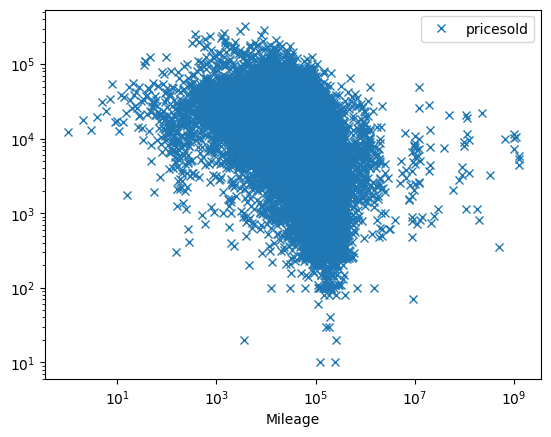
We might wonder how the price is related to the car attributes. Let’s consider it first as a function of milage

Question: Are these correlated?

fix, ax = plt.subplots()
# We take the mean in others
data.pivot_table("pricesold", index="Mileage", aggfunc="mean").plot(
    ax=ax, marker="x", linestyle="none"
)
ax.set_xscale("log")
ax.set_yscale("log")

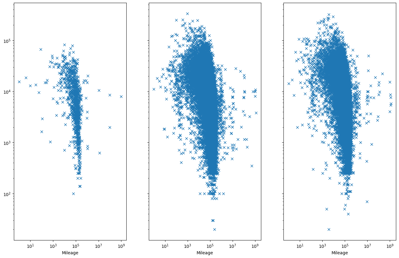
Does it vary with year?

fix, ax = plt.subplots(1, 3, sharey=True, figsize=(16, 10))
# We take the mean in others
tab = data.pivot_table(
    "pricesold", index="Mileage", columns=["yearsold"], aggfunc="mean"
)
for i, year in enumerate((2018, 2019, 2020)):
    tab[year].plot(ax=ax[i], marker="x", linestyle="none")
    ax[i].set_xscale("log")
    ax[i].set_yscale("log")

At this point we would like to see about the role of the cars age. However, we find out there’s something off with the data.

data["Year"].describe()
# We see that we have 92, 0, 20140000

count    1.221440e+05
mean     3.959362e+03
std      1.984514e+05
min      0.000000e+00
25%      1.977000e+03
50%      2.000000e+03
75%      2.008000e+03
max      2.014000e+07
Name: Year, dtype: float64

We show one way of dealing with strangely formated data in the next example. In particular, we will address the problem already when reading the data.

2. People in Norway by region and age in 2022

The dateset is obtained from SSB and we see that the encoding of the age will present some difficulty for numerics.

with open("./data/nor_population2022.csv") as f:
    ln = 0
    while ln < 5:
        print(next(f).strip())
        ln += 1

"region";"alder";"ar";"xxx";"count"
"30 Viken";"000 0 ar";"2022";"Personer";12620
"30 Viken";"001 1 ar";"2022";"Personer";12512
"30 Viken";"002 2 ar";"2022";"Personer";13203
"30 Viken";"003 3 ar";"2022";"Personer";13727

Our solution is to specify a converter for the column which uses regexp to get the age string which is converted to integer

import re

# And we also get rid of some redundant data
data = pd.read_csv(
    "./data/nor_population2022.csv",
    delimiter=";",
    converters={"alder": lambda x: int(re.search(r"(\d+) (ar)", x).group(1))},
).drop(["ar", "xxx"], axis="columns")
data

	region	alder	count
0	30 Viken	0	12620
1	30 Viken	1	12512
2	30 Viken	2	13203
3	30 Viken	3	13727
4	30 Viken	4	14003
...	...	...	...
1267	21 Svalbard	101	0
1268	21 Svalbard	102	0
1269	21 Svalbard	103	0
1270	21 Svalbard	104	0
1271	21 Svalbard	105	0

1272 rows × 3 columns

Question: Can you now fix the problem with car dataset?

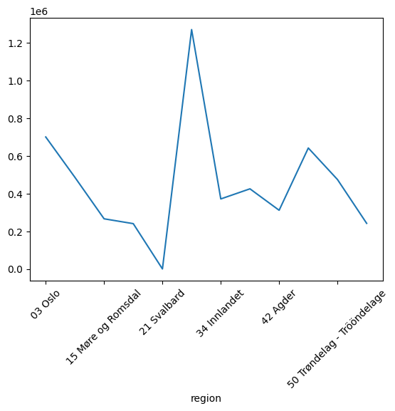
We can have a look at the populaton in different regions

data.groupby("region")["count"].sum().plot()
plt.xticks(rotation=45);

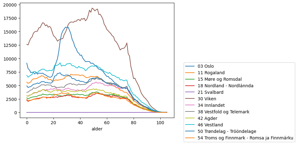
Or breakdown the distribution

fig, ax = plt.subplots()
data.pivot_table("count", index="alder", columns=["region"]).plot(ax=ax)
ax.legend(bbox_to_anchor=(1.05, 0.5))

<matplotlib.legend.Legend at 0x7f8a493da880>

3. Joining

This example is adopted from * Python Data Science Handbook by Jake VanderPlas. We first download the datasets

for name in "abbrevs", "areas", "population":
    fname = f"state-{name}.csv"
    download_file(
        f"data/{fname}",
        url=f"https://raw.githubusercontent.com/jakevdp/data-USstates/HEAD/{fname}",
    )

You can see that they contain data [full name -> population], [full_name -> area], [abbreviation -> full_name]. Given this we want to order the stated by population density

abbrevs = pd.read_csv("./data/state-abbrevs.csv")
areas = pd.read_csv("./data/state-areas.csv")
pop = pd.read_csv("./data/state-population.csv")
abbrevs.head(10)

	state	abbreviation
0	Alabama	AL
1	Alaska	AK
2	Arizona	AZ
3	Arkansas	AR
4	California	CA
5	Colorado	CO
6	Connecticut	CT
7	Delaware	DE
8	District of Columbia	DC
9	Florida	FL

(areas.columns, pop.columns, abbrevs.columns)

(Index(['state', 'area (sq. mi)'], dtype='object'),
 Index(['state/region', 'ages', 'year', 'population'], dtype='object'),
 Index(['state', 'abbreviation'], dtype='object'))

We want to build a table which has both areas and population info. To get there population should get abbreviation so that we can look up areas.

merged = pd.merge(
    pop, abbrevs, left_on="state/region", right_on="abbreviation", how="outer"
).drop("abbreviation", axis=1)
merged.head(5)

	state/region	ages	year	population	state
0	AL	under18	2012	1117489.0	Alabama
1	AL	total	2012	4817528.0	Alabama
2	AL	under18	2010	1130966.0	Alabama
3	AL	total	2010	4785570.0	Alabama
4	AL	under18	2011	1125763.0	Alabama

We inspect the integrity of dataset. Something is wrong with state/region which is a problem if we want to map further.

merged.isnull().any()

state/region    False
ages            False
year            False
population       True
state            True
dtype: bool

By further inspection the missing data is for “not the usual 50 states” and so we just drop them

merged.loc[merged["state"].isnull(), "state/region"].unique()

array(['PR', 'USA'], dtype=object)

merged.dropna(inplace=True)

We can add to our table (left merge) the areas

final = pd.merge(merged, areas, on="state")
final.head(5)

	state/region	ages	year	population	state	area (sq. mi)
0	AL	under18	2012	1117489.0	Alabama	52423
1	AL	total	2012	4817528.0	Alabama	52423
2	AL	under18	2010	1130966.0	Alabama	52423
3	AL	total	2010	4785570.0	Alabama	52423
4	AL	under18	2011	1125763.0	Alabama	52423

We use query (SQL like) language to get the right rows

table = final.query(
    "year == 2012 & ages == 'total'"
)  # final['population']/final['area (sq. mi)']
table.head(10)

	state/region	ages	year	population	state	area (sq. mi)
1	AL	total	2012	4817528.0	Alabama	52423
95	AK	total	2012	730307.0	Alaska	656425
97	AZ	total	2012	6551149.0	Arizona	114006
191	AR	total	2012	2949828.0	Arkansas	53182
193	CA	total	2012	37999878.0	California	163707
287	CO	total	2012	5189458.0	Colorado	104100
289	CT	total	2012	3591765.0	Connecticut	5544
383	DE	total	2012	917053.0	Delaware	1954
385	DC	total	2012	633427.0	District of Columbia	68
479	FL	total	2012	19320749.0	Florida	65758

We will use the states to index into the column. By index preservation this will give us states to density

table.set_index("state", inplace=True)
density = table["population"] / table["area (sq. mi)"]
density.head(5)

state
Alabama        91.897221
Alaska          1.112552
Arizona        57.463195
Arkansas       55.466662
California    232.121278
dtype: float64

density.sort_values(ascending=False).head(10)

state
District of Columbia    9315.102941
New Jersey              1016.710502
Rhode Island             679.808414
Connecticut              647.865260
Massachusetts            629.588157
Maryland                 474.318369
Delaware                 469.320880
New York                 359.359798
Florida                  293.815946
Pennsylvania             277.139151
dtype: float64

Question: Similar data can be obtained from Eurostat. The new thing is that the format .tsv. Let’s start parsing the population data

with open("./data/eustat_population.tsv") as f:
    ln = 0
    while ln < 10:
        print(next(f).strip())
        ln += 1

unit,age,sex,geo\time	2010 	2011 	2012 	2013 	2014 	2015 	2016 	2017 	2018 	2019 	2020 	2021
NR,TOTAL,T,AL01	: 	: 	: 	: 	: 	: 	848059 	826904 	819793 	813758 	804689 	797955
NR,TOTAL,T,AL02	: 	: 	: 	: 	: 	: 	1110562 	1146183 	1162544 	1170142 	1176240 	1178435
NR,TOTAL,T,AL03	: 	: 	: 	: 	: 	: 	927405 	903504 	887987 	878527 	865026 	853351
NR,TOTAL,T,ALXX	: 	: 	: 	: 	: 	: 	: 	: 	0 	0 	: 	:
NR,TOTAL,T,AT11	283697 	284581 	285782 	286691 	287416 	288356 	291011 	291942 	292675 	293433 	294436 	296010
NR,TOTAL,T,AT12	1605897 	1609474 	1614455 	1618592 	1625485 	1636778 	1653691 	1665753 	1670668 	1677542 	1684287 	1690879
NR,TOTAL,T,AT13	1689995 	1702855 	1717084 	1741246 	1766746 	1797337 	1840226 	1867582 	1888776 	1897491 	1911191 	1920949
NR,TOTAL,T,AT21	557998 	556718 	556027 	555473 	555881 	557641 	560482 	561077 	560898 	560939 	561293 	562089
NR,TOTAL,T,AT22	1205045 	1206611 	1208696 	1210971 	1215246 	1221570 	1232012 	1237298 	1240214 	1243052 	1246395 	1247077

We see that the countries are subdivided. Let’s figure out the reader to help here

d = pd.read_csv(
    "./data/eustat_population.tsv",
    sep="\t",
    converters={0: lambda x: re.search(r"([A-Z]{2})(\w\w)$", x).group(1)},
)
d

	unit,age,sex,geo\time	2010	2011	2012	2013	2014	2015	2016	2017	2018	2019	2020	2021
0	AL	:	:	:	:	:	:	848059	826904	819793	813758	804689	797955
1	AL	:	:	:	:	:	:	1110562	1146183	1162544	1170142	1176240	1178435
2	AL	:	:	:	:	:	:	927405	903504	887987	878527	865026	853351
3	AL	:	:	:	:	:	:	:	:	0	0	:	:
4	AT	283697	284581	285782	286691	287416	288356	291011	291942	292675	293433	294436	296010
...	...	...	...	...	...	...	...	...	...	...	...	...	...
337	UK	463388	465794	466605	466737	467326	467889	468903	469420	470743	470990	:	:
338	UK	:	:	1915517	1924614	1933992	1946564	1961928	1976392	1988307	1998699	:	:
339	UK	:	:	1499887	1500987	1504303	1510438	1520628	1531216	1536415	1541998	:	:
340	UK	:	:	946492	945666	944842	944507	945233	946372	946837	947186	:	:
341	UK	1799019	1809539	1818995	1826761	1835290	1846229	1857048	1866638	1875957	:	:	:

342 rows × 13 columns

The next challenge is to handle the missing values which do not show with d.isna() as all the values are strings and the missing is “: “. How would you solve this issue?

4. Timeseries analysis

Our final examples follows Chapter 4. in PDSH. We will be looking at statics from sensors counting bikers on a bridge. We have 2 counters one for left/right side each.

download_file(
    "data/FremontBridge.csv",
    url="https://data.seattle.gov/api/views/65db-xm6k/rows.csv?accessType=DOWNLOAD",
)
data = pd.read_csv("data/FremontBridge.csv", index_col="Date", parse_dates=True)
data.head()

/tmp/ipykernel_419026/796841783.py:5: UserWarning: Could not infer format, so each element will be parsed individually, falling back to `dateutil`. To ensure parsing is consistent and as-expected, please specify a format.
  data = pd.read_csv("data/FremontBridge.csv", index_col="Date", parse_dates=True)

	Fremont Bridge Sidewalks, south of N 34th St	Fremont Bridge Sidewalks, south of N 34th St Cyclist East Sidewalk	Fremont Bridge Sidewalks, south of N 34th St Cyclist West Sidewalk
Date
2022-08-01 00:00:00	23.0	7.0	16.0
2022-08-01 01:00:00	12.0	5.0	7.0
2022-08-01 02:00:00	3.0	0.0	3.0
2022-08-01 03:00:00	5.0	2.0	3.0
2022-08-01 04:00:00	10.0	2.0	8.0

len(data)

95640

For the next steps we will only consider the total count of bikers so we simplify the table

data.columns = ["Total", "East", "West"]
data.drop("East", axis="columns", inplace=True)
data.drop("West", axis="columns", inplace=True)
data

	Total
Date
2022-08-01 00:00:00	23.0
2022-08-01 01:00:00	12.0
2022-08-01 02:00:00	3.0
2022-08-01 03:00:00	5.0
2022-08-01 04:00:00	10.0
...	...
2023-08-31 19:00:00	224.0
2023-08-31 20:00:00	142.0
2023-08-31 21:00:00	67.0
2023-08-31 22:00:00	43.0
2023-08-31 23:00:00	12.0

95640 rows × 1 columns

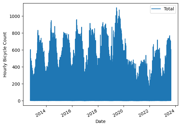
Marking at the data we can definitely see Covid19 but also some seasonal variations

data.plot()
plt.ylabel("Hourly Bicycle Count");  # NOTE: that hour data is for every hour

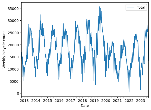
We can downsample the signal to reveal the variations within year better. Below we downsample to Weeks

weekly = data.resample("W").sum()
# Confirmation
weekly.index

DatetimeIndex(['2012-10-07', '2012-10-14', '2012-10-21', '2012-10-28',
               '2012-11-04', '2012-11-11', '2012-11-18', '2012-11-25',
               '2012-12-02', '2012-12-09',
               ...
               '2023-07-02', '2023-07-09', '2023-07-16', '2023-07-23',
               '2023-07-30', '2023-08-06', '2023-08-13', '2023-08-20',
               '2023-08-27', '2023-09-03'],
              dtype='datetime64[ns]', name='Date', length=570, freq='W-SUN')

# And again
weekly.index.isocalendar().week

Date
2012-10-07    40
2012-10-14    41
2012-10-21    42
2012-10-28    43
2012-11-04    44
              ..
2023-08-06    31
2023-08-13    32
2023-08-20    33
2023-08-27    34
2023-09-03    35
Freq: W-SUN, Name: week, Length: 570, dtype: UInt32

weekly.plot(style=["-"])
plt.ylabel("Weekly bicycle count");

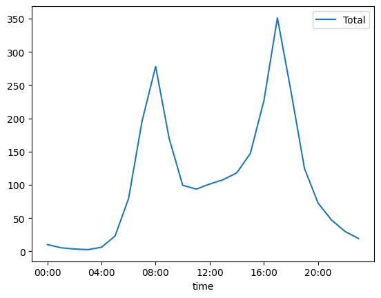
Recall that having time series as index enables many convience functions. For example, we can group/bin data time points by hour and reduce on the subindices giving hous an hourly mean bike usage. It appears to correlate well with rush hours.

by_time = data.groupby(data.index.time).mean()
hourly_ticks = 4 * 60 * 60 * np.arange(6)  # 3600 * 24, every 4 hour
by_time.plot(xticks=hourly_ticks, style=["-"]);

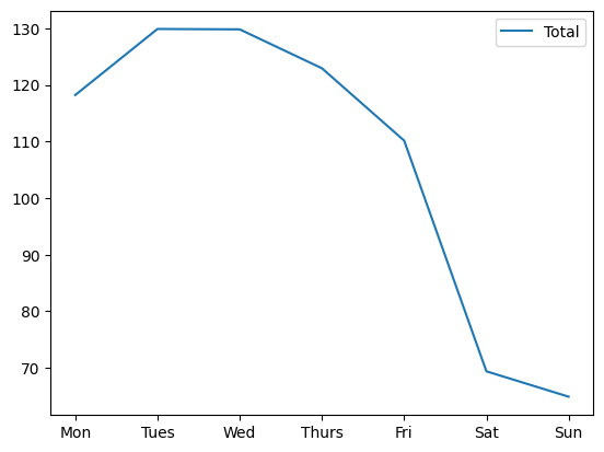
We can repeat the same exercise, this time breaking up the data by hours to reveal that bikes are probably most used for commuting to work

by_weekday = data.groupby(data.index.dayofweek).mean()
by_weekday.index = ["Mon", "Tues", "Wed", "Thurs", "Fri", "Sat", "Sun"]
by_weekday.plot(style=["-"]);

Another look at the same thing using pivot_table

import matplotlib.colors as colors

Z = data.pivot_table(
    "Total", index=data.index.weekday, columns=[data.index.time]
).values

plt.pcolor(Z, norm=colors.LogNorm(vmin=Z.min(), vmax=Z.max()), cmap="inferno")
plt.colorbar()

<matplotlib.colorbar.Colorbar at 0x7f8a46820460>

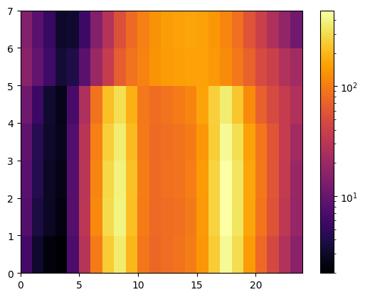
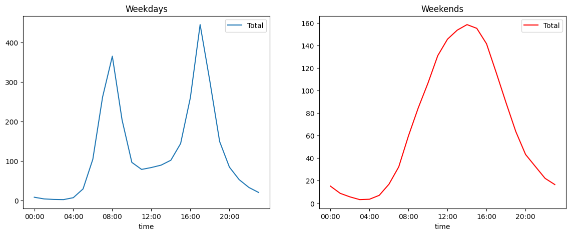
The heatmap suggests that there are 2 peaks in weekdays and a single one during the weekend. We can varify this by essentially collapsing/averaging the plot in the vertical direction separately for the two categories of days. Let’s compute the mask for each day in the series

weekend = np.where(data.index.weekday < 5, "Weekday", "Weekend")

Using the mask we can group the data first by the day catogory and then by hours

by_time = data.groupby([weekend, data.index.time]).mean()
by_time.index[:4]

MultiIndex([('Weekday', 00:00:00),
            ('Weekday', 01:00:00),
            ('Weekday', 02:00:00),
            ('Weekday', 03:00:00)],
           )

Finally we have the two collapsed plots

import matplotlib.pyplot as plt

fig, ax = plt.subplots(1, 2, figsize=(14, 5))
by_time.loc["Weekday"].plot(
    ax=ax[0], title="Weekdays", xticks=hourly_ticks, style=["-"]
)
by_time.loc["Weekend"].plot(
    ax=ax[1], title="Weekends", xticks=hourly_ticks, style=["-"], color="red"
);

Question: Head on to Oslo Bysykkel web and get the trip data (as CSV). In the last years the students analyzed the trips by distance (see the IN3110 course webpage). What about the distribution of trips by the average speed? Can you use this to infer if the trip was going (on average) uphill or downhill?

bike_csv = "./data/oslo_bike_2022_09.csv"
download_file(
    bike_csv, url="https://data.urbansharing.com/oslobysykkel.no/trips/v1/2022/09.csv"
)

PosixPath('data/oslo_bike_2022_09.csv')

with open(bike_csv) as f:
    print(next(f).strip())
    print(next(f).strip())

started_at,ended_at,duration,start_station_id,start_station_name,start_station_description,start_station_latitude,start_station_longitude,end_station_id,end_station_name,end_station_description,end_station_latitude,end_station_longitude
2022-09-01 03:04:31.178000+00:00,2022-09-01 03:13:01.298000+00:00,510,437,Sentrum Scene,ved Arbeidersamfunnets plass,59.91546786564256,10.751140873016311,583,Galgeberg,langs St. Halvards gate,59.90707579234818,10.779164402446728

At this point we know that time info should be parsed with dates. For duration (in seconds) we will have ints

data = pd.read_csv(
    bike_csv,
    parse_dates=["started_at", "ended_at"],
    dtype={"duration": int},
)
data.head(5)

	started_at	ended_at	duration	start_station_id	start_station_name	start_station_description	start_station_latitude	start_station_longitude	end_station_id	end_station_name	end_station_description	end_station_latitude	end_station_longitude
0	2022-09-01 03:04:31.178000+00:00	2022-09-01 03:13:01.298000+00:00	510	437	Sentrum Scene	ved Arbeidersamfunnets plass	59.915468	10.751141	583	Galgeberg	langs St. Halvards gate	59.907076	10.779164
1	2022-09-01 03:11:09.104000+00:00	2022-09-01 03:14:52.506000+00:00	223	578	Hallings gate	langs Dalsbergstien	59.922777	10.738655	499	Bjerregaards gate	ovenfor Fredrikke Qvams gate	59.925488	10.746058
2	2022-09-01 03:11:37.861000+00:00	2022-09-01 03:23:23.939000+00:00	706	421	Alexander Kiellands Plass	langs Maridalsveien	59.928067	10.751203	390	Saga Kino	langs Olav Vs gate	59.914240	10.732771
3	2022-09-01 03:13:00.843000+00:00	2022-09-01 03:17:17.639000+00:00	256	735	Oslo Hospital	ved trikkestoppet	59.903213	10.767344	465	Bjørvika	under broen Nylandsveien	59.909006	10.756180
4	2022-09-01 03:13:13.330000+00:00	2022-09-01 03:24:15.758000+00:00	662	525	Myraløkka Øst	ved Bentsenbrua	59.937205	10.760581	443	Sjøsiden ved trappen	Oslo S	59.910154	10.751981

What is the station with most departures?

data["start_station_id"].value_counts().sort_values(ascending=False)

start_station_id
421     2133
1755    2079
480     1984
398     1970
551     1918
        ... 
591       84
1919      74
454       72
560       58
573       44
Name: count, Length: 263, dtype: int64

We will approximate the trip distance by measing it as the geodesic between start and end points.

from math import asin, cos, pi, sin, sqrt


def trip_distance(row):
    """As the crow flies"""
    lat_station = row["start_station_latitude"]
    lon_station = row["start_station_longitude"]

    lat_sentrum = row["end_station_latitude"]
    lon_sentrum = row["end_station_longitude"]

    degrees = pi / 180  # convert degrees to radians
    a = (
        0.5
        - (cos((lat_sentrum - lat_station) * degrees) / 2)
        + (
            cos(lat_sentrum * degrees)
            * cos(lat_station * degrees)
            * (1 - cos((lon_station - lon_sentrum) * degrees))
            / 2
        )
    )
    # We have the return value in meters
    return 12742_000 * asin(sqrt(a))  # 2 * R * asin...


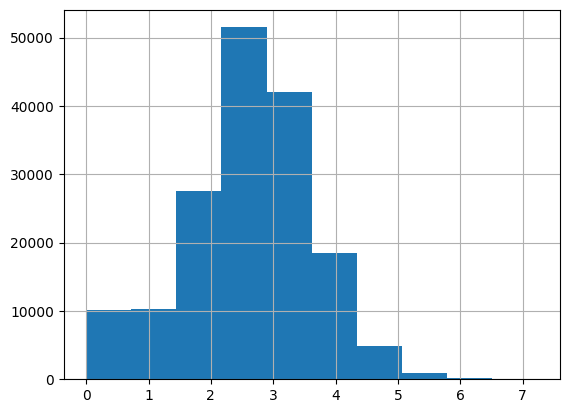
distance = data.apply(trip_distance, axis="columns")

duration = data["duration"]
speed = distance / duration

speed.hist()

<AxesSubplot: >

Bonus: Visualization

from ipyleaflet import Circle, Map, Marker, Polyline, basemap_to_tiles, basemaps
from ipywidgets import HTML

trip_csv = "./data/oslo_bike_2022_09.csv"
trips = pd.read_csv(trip_csv)
station_data = trips.groupby(
    [
        "start_station_id",
        "start_station_longitude",
        "start_station_latitude",
        "start_station_name",
    ]
).count()
station_data = station_data.reset_index()
station_data = station_data.drop(columns=station_data.columns[-7:])
station_data = station_data.rename(columns={"started_at": "started_trips"})
station_data = station_data.set_index("start_station_id")
station_data["ended_trips"] = trips["end_station_id"].value_counts()

oslo_center = (
    59.9127,
    10.7461,
)  # NB ipyleaflet uses Lat-Long (i.e. y,x, when specifying coordinates)
oslo_map = Map(center=oslo_center, zoom=13, close_popup_on_click=False)


def add_markers(row):
    center = row["start_station_latitude"], row["start_station_longitude"]
    marker = Marker(location=center)
    marker2 = Circle(
        location=center, radius=int(0.04 * row["ended_trips"]), color="red"
    )

    message = HTML()
    message.value = (
        f"{row['start_station_name']} <br> Trips started: {row['started_trips']}"
    )

    marker.popup = message
    oslo_map.add_layer(marker)
    oslo_map.add_layer(marker2)


station_data.apply(add_markers, axis=1)

start_station_id
377     None
378     None
380     None
381     None
382     None
        ... 
2340    None
2347    None
2349    None
2350    None
2351    None
Length: 263, dtype: object

oslo_map